|
Size: 16254
Comment: Summarize #6162
|
Size: 25258
Comment: Summarize #3084, #6097, #6417, #5637
|
| Deletions are marked like this. | Additions are marked like this. |
| Line 332: | Line 332: |
| {{{ | {{{#!python numbers=off |
| Line 340: | Line 340: |
| {{{ | {{{#!python numbers=off |
| Line 345: | Line 345: |
| {{{ | {{{#!python numbers=off |
| Line 351: | Line 351: |
| == Group Theory == == Interfaces == * FIXME: summarize #4313 |
|
| Line 363: | Line 354: |
| * FIXME: summarize #6261 * FIXME: summarize #5882 |
* Multiplicative order for matrices over finite fields (Yann Laigle-Chapuy) -- New method {{{multiplicative_order()}}} in the class {{{Matrix}}} of {{{sage/matrix/matrix0.pyx}}} for computing the multiplicative order of a matrix. Here are some examples on using the new method {{{multiplicative_order()}}}: {{{#!python numbers=off sage: A = matrix(GF(59), 3, [10,56,39,53,56,33,58,24,55]) sage: A.multiplicative_order() 580 sage: (A^580).is_one() True sage: B = matrix(GF(10007^3, 'b'), 0) sage: B.multiplicative_order() 1 sage: E = MatrixSpace(GF(11^2, 'e'), 5).random_element() sage: (E^E.multiplicative_order()).is_one() True }}} * A general package for finitely generated not-necessarily free R-modules (William Stein, David Loeffler ) -- This consists of the following new Sage modules: * {{{sage/modules/fg_pid/fgp_element.py}}} -- Elements of finitely generated modules over a principal ideal domain. Here are some examples: {{{#!python numbers=off sage: V = span([[1/2,1,1], [3/2,2,1], [0,0,1]], ZZ) sage: W = V.span([2*V.0+4*V.1, 9*V.0+12*V.1, 4*V.2]) sage: Q = V/W sage: x = Q(V.0-V.1); x (0, 3) sage: type(x) <class 'sage.modules.fg_pid.fgp_element.FGP_Element'> sage: x is Q(x) True sage: x.parent() is Q True sage: Q Finitely generated module V/W over Integer Ring with invariants (4, 12) sage: Q.0.additive_order() 4 sage: Q.1.additive_order() 12 sage: (Q.0+Q.1).additive_order() 12 }}} * {{{sage/modules/fg_pid/fgp_module.py}}} -- Finitely generated modules over a principal ideal domain. Currently, on the principal ideal domain {{{ZZ}}} of integers is supported. Here are some examples: {{{#!python numbers=off sage: V = span([[1/2,1,1], [3/2,2,1], [0,0,1]], ZZ) sage: W = V.span([2*V.0+4*V.1, 9*V.0+12*V.1, 4*V.2]) sage: import sage.modules.fg_pid.fgp_module sage: Q = sage.modules.fg_pid.fgp_module.FGP_Module(V, W) sage: type(Q) <class 'sage.modules.fg_pid.fgp_module.FGP_Module_class'> sage: Q is sage.modules.fg_pid.fgp_module.FGP_Module(V, W, check=False) True sage: X = ZZ**2 / span([[3,0],[0,2]], ZZ) sage: X.linear_combination_of_smith_form_gens([1]) (1) sage: Q Finitely generated module V/W over Integer Ring with invariants (4, 12) sage: Q.gens() ((1, 0), (0, 1)) sage: Q.coordinate_vector(-Q.0) (-1, 0) sage: Q.coordinate_vector(-Q.0, reduce=True) (3, 0) sage: Q.cardinality() 48 }}} * {{{sage/modules/fg_pid/fgp_morphism.py}}} -- Morphisms between finitely generated modules over a principal ideal domain. Here are some examples: {{{#!python numbers=off sage: V = span([[1/2,1,1],[3/2,2,1],[0,0,1]],ZZ) sage: W = V.span([2*V.0+4*V.1, 9*V.0+12*V.1, 4*V.2]) sage: Q = V/W; Q Finitely generated module V/W over Integer Ring with invariants (4, 12) sage: phi = Q.hom([Q.0+3*Q.1, -Q.1]); phi Morphism from module over Integer Ring with invariants (4, 12) to module with invariants (4, 12) that sends the generators to [(1, 3), (0, 11)] sage: phi(Q.0) == Q.0 + 3*Q.1 True sage: phi(Q.1) == -Q.1 True sage: Q.hom([0, Q.1]).kernel() Finitely generated module V/W over Integer Ring with invariants (4) sage: A = Q.hom([Q.0, 0]).kernel(); A Finitely generated module V/W over Integer Ring with invariants (12) sage: Q.1 in A True sage: phi = Q.hom([Q.0-3*Q.1, Q.0+Q.1]) sage: A = phi.kernel(); A Finitely generated module V/W over Integer Ring with invariants (4) sage: phi(A) Finitely generated module V/W over Integer Ring with invariants () }}} |
| Line 370: | Line 449: |
| * FIXME: summarize #3084 * FIXME: summarize #6097 * FIXME: summarize #6417 == Modular Forms == |
* An optimized Sudoku solver (Rob Beezer, Tom Boothby) -- Support two algorithms for efficiently solving a Sudoku puzzle: a backtrack algorithm and the DLX algorithm. Generally, the DLX algorithm is very fast and very consistent. The backtrack algorithm is very variable in its performance, on some occasions markedly faster than DLX but usually slower by a similar factor, with the potential to be orders of magnitude slower. The following, we compare the performance between the Sudoku solver in Sage 4.0.2 and that in this release. We also compare the performance between the backtrack algorithm and the DLX algorithm. All timing statistics were obtained using the machine sage.math: {{{#!python numbers=off # BEFORE sage: A = matrix(ZZ,9,[5,0,0, 0,8,0, 0,4,9, 0,0,0, 5,0,0, 0,3,0, 0,6,7, \ ....: 3,0,0, 0,0,1, 1,5,0, 0,0,0, 0,0,0, 0,0,0, 2,0,8, 0,0,0, \ ....: 0,0,0, 0,0,0, 0,1,8, \ ....: 7,0,0, 0,0,4, 1,5,0, 0,3,0, 0,0,2, 0,0,0, 4,9,0, 0,5,0, 0,0,3]) sage: %timeit sudoku(A); 10 loops, best of 3: 43.5 ms per loop sage: from sage.games.sudoku import solve_recursive sage: B = matrix(ZZ, 9, 9, [ [0,0,0,0,1,0,9,0,0], [8,0,0,4,0,0,0,0,0], \ ....: [2,0,0,0,0,0,0,0,0], [0,7,0,0,3,0,0,0,0], [0,0,0,0,0,0,2,0,4], \ ....: [0,0,0,0,0,0,0,5,8], [0,6,0,0,0,0,1,3,0], [7,0,0,2,0,0,0,0,0], \ ....: [0,0,0,8,0,0,0,0,0] ]) sage: %timeit solve_recursive(B, 8, 5); 1000 loops, best of 3: 325 µs per loop # AFTER sage: h = Sudoku('8..6..9.5.............2.31...7318.6.24.....73...........279.1..5...8..36..3......') sage: %timeit h.solve(algorithm='backtrack').next(); 1000 loops, best of 3: 1.12 ms per loop sage: %timeit h.solve(algorithm='dlx').next(); 1000 loops, best of 3: 1.58 ms per loop sage: # These are the first 10 puzzles in a list of "Top 95" puzzles. sage: top =['4.....8.5.3..........7......2.....6.....8.4......1.......6.3.7.5..2.....1.4......',\ ....: '52...6.........7.13...........4..8..6......5...........418.........3..2...87.....',\ ....: '6.....8.3.4.7.................5.4.7.3..2.....1.6.......2.....5.....8.6......1....',\ ....: '48.3............71.2.......7.5....6....2..8.............1.76...3.....4......5....',\ ....: '....14....3....2...7..........9...3.6.1.............8.2.....1.4....5.6.....7.8...',\ ....: '......52..8.4......3...9...5.1...6..2..7........3.....6...1..........7.4.......3.',\ ....: '6.2.5.........3.4..........43...8....1....2........7..5..27...........81...6.....',\ ....: '.524.........7.1..............8.2...3.....6...9.5.....1.6.3...........897........',\ ....: '6.2.5.........4.3..........43...8....1....2........7..5..27...........81...6.....',\ ....: '.923.........8.1...........1.7.4...........658.........6.5.2...4.....7.....9.....'] sage: p = [Sudoku(top[i]) for i in xrange(10)] sage: for i in xrange(10): ....: %timeit p[i].solve(algorithm='dlx').next(); ....: %timeit p[i].solve(algorithm='backtrack').next(); ....: 100 loops, best of 3: 2.26 ms per loop 10 loops, best of 3: 223 ms per loop 100 loops, best of 3: 2.6 ms per loop 10 loops, best of 3: 21.3 ms per loop 100 loops, best of 3: 2.38 ms per loop 10 loops, best of 3: 83.5 ms per loop 1000 loops, best of 3: 1.76 ms per loop 10 loops, best of 3: 43.5 ms per loop 1000 loops, best of 3: 1.86 ms per loop 10 loops, best of 3: 316 ms per loop 1000 loops, best of 3: 1.65 ms per loop 10 loops, best of 3: 145 ms per loop 100 loops, best of 3: 1.84 ms per loop 10 loops, best of 3: 547 ms per loop 1000 loops, best of 3: 1.77 ms per loop 10 loops, best of 3: 255 ms per loop 100 loops, best of 3: 2.08 ms per loop 10 loops, best of 3: 445 ms per loop 1000 loops, best of 3: 1.67 ms per loop 10 loops, best of 3: 266 ms per loop }}} * A decorator for declaring abstract methods (Nicolas Thiéry) -- Support a decorator that can be used to declare a method that should be implemented by derived classes. This declaration should typically include documentation for the specification for this method. The purpose of the decorator is to enforce a consistent and visual syntax for such declarations. The decorator is also used by the Sage categories framework for automated tests. As an example, here we create a class with an abstract method: {{{#!python numbers=off sage: class A(object): ....: @abstract_method ....: def my_method(self): ....: """ ....: The method :meth:`my_method` computes my_method ....: """ ....: pass ....: sage: A.my_method <abstract method my_method at 0x7f53414a7410> }}} The current policy is that a {{{NotImplementedError}}} is raised when accessing the method through an instance, even before the method is called: {{{#!python numbers=off sage: x = A() sage: x.my_method Traceback (most recent call last): ... NotImplementedError: <abstract method my_method at 0x7f53414a7410> }}} It is also possible to mark abstract methods as optional: {{{#!python numbers=off sage: class A(object): ....: @abstract_method(optional=True) ....: def my_method(self): ....: """ ....: The method :meth:`my_method` computes my_method ....: """ ....: pass ....: sage: A.my_method <optional abstract method my_method at 0x3b551b8> sage: x = A() sage: x.my_method NotImplemented }}} |
| Line 383: | Line 556: |
| * FIXME: summarize #5637 | * Unicode in {{{%latex}}} cells (Peter Mora) -- One can now enter Unicode characters directly in Notebook cells. Here is a screenshot illustrating this: {{attachment:unicode-latex.png}} * Allow {{{\[}}} and {{{\]}}} to delimit math in {{{%html}}} blocks (John Palmieri) -- One can now enter {{{#!python numbers=off %html test \[ x^2 \] }}} and the expression {{{x^2}}} is typeset in math mode. |
Sage 4.1 Release Tour
Sage 4.1 was released on July 09, 2009. For the official, comprehensive release note, please refer to sage-4.1.txt. A nicely formatted version of this release tour can be found at FIXME. The following points are some of the foci of this release:
- Upgrade to Python 2.6.x
- Support for building Singular with GCC 4.4
- Optimized integer division
- Combinatorics: irreducible matrix representations of symmetric groups; and Yang-Baxter Graphs
- Cryptography: Mini Advanced Encryption Standard for educational purposes
- Graph theory: back-end for graph theory with Cython (c_graph); and improve accuracy of graph eigenvalues
- Linear algebra: a general package for finitely generated, not-necessarily free R-modules; and multiplicative order for matrices over finite fields
- Miscellaneous: optimized Sudoku solver; a decorator for declaring abstract methods; and support Unicode in LaTeX cells (notebook)
- Number theory: improved random element generation for number field orders and ideals; support Michael Stoll's ratpoints package; and elliptic exponential
- Numerical: computing numerical values of constants using mpmath
- Update, upgrade 18 packages to latest upstream releases
Algebraic Geometry
Construct an elliptic curve from a plane curve of genus one (Lloyd Kilford, John Cremona ) -- New function EllipticCurve_from_plane_curve() in the module sage/schemes/elliptic_curves/constructor.py to allow the construction of an elliptic curve from a smooth plane cubic with a rational point. Currently, this function uses Magma and it will not work on machines that do not have Magma installed. Assuming you have Magma installed on your computer, we can use the function EllipticCurve_from_plane_curve() to first check that the Fermat cubic is isomorphic to the curve with Cremona label "27a1":
Here is a quartic example:sage: x, y, z = PolynomialRing(QQ, 3, 'xyz').gens() # optional - magma sage: C = Curve(x^3 + y^3 + z^3) # optional - magma sage: P = C(1, -1, 0) # optional - magma sage: E = EllipticCurve_from_plane_curve(C, P) # optional - magma sage: E # optional - magma Elliptic Curve defined by y^2 + y = x^3 - 7 over Rational Field sage: E.label() # optional - magma '27a1'
sage: u, v, w = PolynomialRing(QQ, 3, 'uvw').gens() # optional - magma
sage: C = Curve(u^4 + u^2*v^2 - w^4) # optional - magma
sage: P = C(1, 0, 1) # optional - magma
sage: E = EllipticCurve_from_plane_curve(C, P) # optional - magma
sage: E # optional - magma
Elliptic Curve defined by y^2  = x^3 + 4*x over Rational Field
sage: E.label() # optional - magma
'32a1'
Basic Arithmetic
- Speed-up integer division (Robert Bradshaw ) -- In some cases, integer division is now up to 31% faster than previously. The following timing statistics were obtained using the machine sage.math:
# BEFORE

sage: a = next_prime(2**31)
sage: b = Integers(a)(100)
sage: %timeit a % b;
1000000 loops, best of 3: 1.12 µs per loop
sage: %timeit 101 // int(5);
1000000 loops, best of 3: 215 ns per loop
sage: %timeit 100 // int(-3)
1000000 loops, best of 3: 214 ns per loop
sage: a = ZZ.random_element(10**50)
sage: b = ZZ.random_element(10**15)
sage: %timeit a.quo_rem(b)
1000000 loops, best of 3: 454 ns per loop


# AFTER

sage: a = next_prime(2**31)
sage: b = Integers(a)(100)
sage: %timeit a % b;
1000000 loops, best of 3: 1.02 µs per loop
sage: %timeit 101 // int(5);
1000000 loops, best of 3: 201 ns per loop
sage: %timeit 100 // int(-3)
1000000 loops, best of 3: 194 ns per loop
sage: a = ZZ.random_element(10**50)
sage: b = ZZ.random_element(10**15)
sage: %timeit a.quo_rem(b)
1000000 loops, best of 3: 313 ns per loop
Combinatorics
Irreducible matrix representations of symmetric groups (Franco Saliola) -- Support for constructing irreducible representations of the symmetric group. This is based on Alain Lascoux's article Young representations of the symmetric group. The following types of representations are supported:
- Specht representations -- The matrices have integer entries:
sage: chi = SymmetricGroupRepresentation([3, 2]); chi
Specht representation of the symmetric group corresponding to [3, 2]
sage: chi([5, 4, 3, 2, 1])

[ 1 -1  0  1  0]
[ 0  0 -1  0  1]
[ 0  0  0 -1  1]
[ 0  1 -1 -1  1]
[ 0  1  0 -1  1]
- Young's seminormal representation -- The matrices have rational entries:
sage: snorm = SymmetricGroupRepresentation([2, 1], "seminormal"); snorm
Seminormal representation of the symmetric group corresponding to [2, 1]
sage: snorm([1, 3, 2])

[-1/2  3/2]
[ 1/2  1/2]
Young's orthogonal representation (the matrices are orthogonal) -- These matrices are defined over Sage's Symbolic Ring:
sage: ortho = SymmetricGroupRepresentation([3, 2], "orthogonal"); ortho
Orthogonal representation of the symmetric group corresponding to [3, 2]
sage: ortho([1, 3, 2, 4, 5])

[          1           0           0           0           0]
[          0        -1/2 1/2*sqrt(3)           0           0]
[          0 1/2*sqrt(3)         1/2           0           0]
[          0           0           0        -1/2 1/2*sqrt(3)]
[          0           0           0 1/2*sqrt(3)         1/2]
You can also create the CombinatorialClass of all irreducible matrix representations of a given symmetric group. Then particular representations can be created by providing partitions. For example:
sage: chi = SymmetricGroupRepresentations(5); chi
Specht representations of the symmetric group of order 5! over Integer Ring
sage: chi([5]) # the trivial representation
Specht representation of the symmetric group corresponding to [5]
sage: chi([5])([2, 1, 3, 4, 5])
[1]
sage: chi([1, 1, 1, 1, 1]) # the sign representation
Specht representation of the symmetric group corresponding to [1, 1, 1, 1, 1]
sage: chi([1, 1, 1, 1, 1])([2, 1, 3, 4, 5])
[-1]
sage: chi([3, 2])
Specht representation of the symmetric group corresponding to [3, 2]
sage: chi([3, 2])([5, 4, 3, 2, 1])

[ 1 -1  0  1  0]
[ 0  0 -1  0  1]
[ 0  0  0 -1  1]
[ 0  1 -1 -1  1]
[ 0  1  0 -1  1]
See the documentation of SymmetricGroupRepresentation and SymmetricGroupRepresentations for more information and examples.
- Specht representations -- The matrices have integer entries:
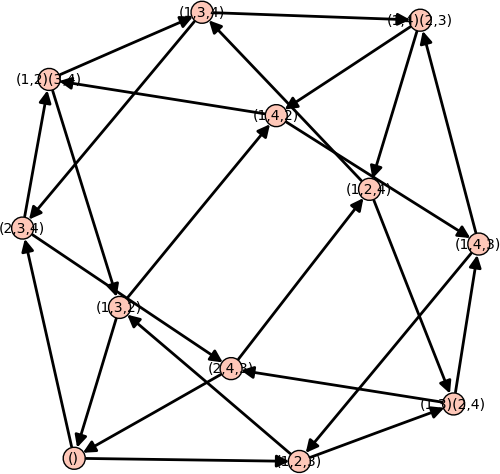
- Yang-Baxter graphs (Franco Saliola) -- Besides being used for constructing the irreducible matrix representations of the symmetric group, Yang-Baxter graphs can also be used to construct the Cayley graph of a finite group. For example:
sage: def left_multiplication_by(g):
....:     return lambda h : h*g
....:
sage: G = AlternatingGroup(4)
sage: operators = [ left_multiplication_by(gen) for gen in G.gens() ]
sage: Y = YangBaxterGraph(root=G.identity(), operators=operators); Y
Yang-Baxter graph with root vertex ()
sage: Y.plot(edge_labels=False)
- Yang-Baxter graphs can also be used to construct the permutahedron:
sage: from sage.combinat.yang_baxter_graph import SwapIncreasingOperator
sage: operators = [SwapIncreasingOperator(i) for i in range(3)]
sage: Y = YangBaxterGraph(root=(1,2,3,4), operators=operators); Y
Yang-Baxter graph with root vertex (1, 2, 3, 4)
sage: Y.plot()
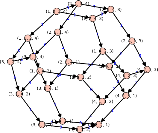
See the documentation of YangBaxterGraph for more information and examples.
Cryptography
Mini Advanced Encryption Standard for educational purposes (Minh Van Nguyen) -- New module sage/crypto/block_cipher/miniaes.py to support the Mini Advanced Encryption Standard (Mini-AES) to allow students to explore the working of a block cipher. This is a simplified variant of the Advanced Encryption Standard (AES) to be used for cryptography education. Mini-AES is described in the paper:
- A. C.-W. Phan. Mini advanced encryption standard (mini-AES): a testbed for cryptanalysis students. Cryptologia, 26(4):283--306, 2002.
Here is the decryption process:sage: from sage.crypto.block_cipher.miniaes import MiniAES sage: maes = MiniAES() sage: K = FiniteField(16, "x") sage: MS = MatrixSpace(K, 2, 2) sage: P = MS([K("x^3 + x"), K("x^2 + 1"), K("x^2 + x"), K("x^3 + x^2")]); P [ x^3 + x x^2 + 1] [ x^2 + x x^3 + x^2] sage: key = MS([K("x^3 + x^2"), K("x^3 + x"), K("x^3 + x^2 + x"), K("x^2 + x + 1")]); key [ x^3 + x^2 x^3 + x] [x^3 + x^2 + x x^2 + x + 1] sage: C = maes.encrypt(P, key); C [ x x^2 + x] [x^3 + x^2 + x x^3 + x]
We can also work directly with binary strings:sage: plaintxt = maes.decrypt(C, key) sage: plaintxt == P True
sage: from sage.crypto.block_cipher.miniaes import MiniAES
sage: maes = MiniAES()
sage: bin = BinaryStrings()
sage: key = bin.encoding("KE"); key
0100101101000101
sage: P = bin.encoding("Encrypt this secret message!")
sage: C = maes(P, key, algorithm="encrypt")
sage: plaintxt = maes(C, key, algorithm="decrypt")
sage: plaintxt == P
True
Or work with integers n such that 0 <= n <= 15:
sage: from sage.crypto.block_cipher.miniaes import MiniAES
sage: maes = MiniAES()
sage: P = [n for n in xrange(16)]; P
[0, 1, 2, 3, 4, 5, 6, 7, 8, 9, 10, 11, 12, 13, 14, 15]
sage: key = [2, 3, 11, 0]; key
[2, 3, 11, 0]
sage: P = maes.integer_to_binary(P)
sage: key = maes.integer_to_binary(key)
sage: C = maes(P, key, algorithm="encrypt")
sage: plaintxt = maes(C, key, algorithm="decrypt")
sage: plaintxt == P
True
Graph Theory
Fast compiled graphs c_graph (Robert Miller) -- The Python package NetworkX version 0.36 is currently the default graph implementation in Sage. The goal of fast compiled graphs, or c_graph, is to be the default implementation of graph theory in Sage. The c_graph implementation is developed using Cython, which allows graph theoretic computations to run at the speed of C. The c_graph backend is implemented in the module sage/graphs/base/c_graph.pyx. This module is called by higher-level frontends in sage/graphs/. Where support is provided for using c_graph, graph theoretic computations is usually more efficient than using NetworkX. For example, the following timing statistics were obtained using the machine sage.math:
# NetworkX 0.36

sage: time G = Graph(1000000, implementation="networkx")
CPU times: user 8.74 s, sys: 0.27 s, total: 9.01 s
Wall time: 9.08 s


# c_graph

sage: time G = Graph(1000000, implementation="c_graph")
CPU times: user 0.01 s, sys: 0.14 s, total: 0.15 s
Wall time: 0.19 s
Here, we see an efficiency gain of up to 47x using c_graph.
- Improve accuracy of graph eigenvalues (Rob Beezer) -- New routines compute eigenvalues and eigenvectors of integer matrices more precisely than before. Rather than convert adjacency matrices of graphs to computations over the real or complex fields, adjacency matrices are retained as matrices over the integers, yielding more accurate and informative results for eigenvalues, eigenvectors, and eigenspaces. Here is a comparison involving the computation of graph spectrum: Integer eigenvalues are now exact, irrational eigenvalues are more precise than previously, making multiplicities easier to determine. Similar comments apply to eigenvectors:
# BEFORE

sage: g = graphs.CycleGraph(8); g
Cycle graph: Graph on 8 vertices
sage: g.spectrum()

[-2.0,
 -1.41421356237,
 -1.41421356237,
 4.02475820828e-18,
 6.70487495185e-17,
 1.41421356237,
 1.41421356237,
 2.0]


# AFTER

sage: g = graphs.CycleGraph(8); g
Cycle graph: Graph on 8 vertices
sage: g.spectrum()
[2, 1.414213562373095?, 1.414213562373095?, 0, 0, -1.414213562373095?, -1.414213562373095?, -2]
sage: g.eigenvectors()

[(2, [
(1, 1, 1, 1, 1, 1, 1, 1)
], 1),
 (-2, [
(1, -1, 1, -1, 1, -1, 1, -1)
], 1),
 (0, [
(1, 0, -1, 0, 1, 0, -1, 0),
(0, 1, 0, -1, 0, 1, 0, -1)
], 2),
 (-1.414213562373095?,
  [(1, 0, -1, 1.414213562373095?, -1, 0, 1, -1.414213562373095?),
   (0, 1, -1.414213562373095?, 1, 0, -1, 1.414213562373095?, -1)],
  2),
 (1.414213562373095?,
  [(1, 0, -1, -1.414213562373095?, -1, 0, 1, 1.414213562373095?),
   (0, 1, 1.414213562373095?, 1, 0, -1, -1.414213562373095?, -1)],
  2)]
Eigenspaces are exact, in that they can be expressed as vector spaces over number fields. When the defining polynomial has several roots, the eigenspaces are not repeated. Previously, eigenspaces were "fractured" owing to slight computational differences in identical eigenvalues. In concert with eigenvectors(), this command illuminates the structure of a graph's eigenspaces more than purely numerical results.
Complex eigenvalues (of digraphs) previously were missing their imaginary parts. This issue has been fixed as part of the improvement in calculating graph eigenvalues.sage: g.eigenspaces() [ (2, Vector space of degree 8 and dimension 1 over Rational Field User basis matrix: [1 1 1 1 1 1 1 1]), (-2, Vector space of degree 8 and dimension 1 over Rational Field User basis matrix: [ 1 -1 1 -1 1 -1 1 -1]), (0, Vector space of degree 8 and dimension 2 over Rational Field User basis matrix: [ 1 0 -1 0 1 0 -1 0] [ 0 1 0 -1 0 1 0 -1]), (a3, Vector space of degree 8 and dimension 2 over Number Field in a3 with defining polynomial x^2 - 2 User basis matrix: [ 1 0 -1 -a3 -1 0 1 a3] [ 0 1 a3 1 0 -1 -a3 -1]) ]
Graphics
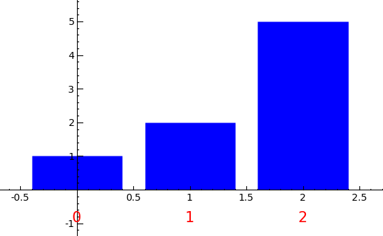
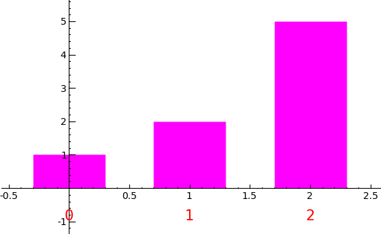
Plot histogram improvement (David Joyner) -- Some improvements to the plot_histogram() function of the class IndexedSequence in sage/gsl/dft.py. The default colour of the histogram is blue:
sage: J = range(3)
sage: A = [ZZ(i^2)+1 for i in J]
sage: s = IndexedSequence(A, J)
sage: s.plot_histogram()
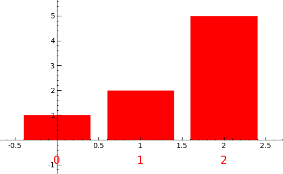
You can now change the colour of the histogram with the argument clr:
sage: s.plot_histogram(clr=(1,0,0))
and even use the argument eps to change the width of the spacing between the bars:
sage: s.plot_histogram(clr=(1,0,1), eps=0.3)
Linear Algebra
Multiplicative order for matrices over finite fields (Yann Laigle-Chapuy) -- New method multiplicative_order() in the class Matrix of sage/matrix/matrix0.pyx for computing the multiplicative order of a matrix. Here are some examples on using the new method multiplicative_order():
sage: A = matrix(GF(59), 3, [10,56,39,53,56,33,58,24,55])
sage: A.multiplicative_order()
580
sage: (A^580).is_one()
True
sage: B = matrix(GF(10007^3, 'b'), 0)
sage: B.multiplicative_order()
1
sage: E = MatrixSpace(GF(11^2, 'e'), 5).random_element()
sage: (E^E.multiplicative_order()).is_one()
True
- A general package for finitely generated not-necessarily free R-modules (William Stein, David Loeffler ) -- This consists of the following new Sage modules:
sage/modules/fg_pid/fgp_element.py -- Elements of finitely generated modules over a principal ideal domain. Here are some examples:
sage: V = span([[1/2,1,1], [3/2,2,1], [0,0,1]], ZZ)
sage: W = V.span([2*V.0+4*V.1, 9*V.0+12*V.1, 4*V.2])
sage: Q = V/W
sage: x = Q(V.0-V.1); x
(0, 3)
sage: type(x)
<class 'sage.modules.fg_pid.fgp_element.FGP_Element'>
sage: x is Q(x)
True
sage: x.parent() is Q
True
sage: Q
Finitely generated module V/W over Integer Ring with invariants (4, 12)
sage: Q.0.additive_order()
4
sage: Q.1.additive_order()
12
sage: (Q.0+Q.1).additive_order()
12
sage/modules/fg_pid/fgp_module.py -- Finitely generated modules over a principal ideal domain. Currently, on the principal ideal domain ZZ of integers is supported. Here are some examples:
sage: V = span([[1/2,1,1], [3/2,2,1], [0,0,1]], ZZ)
sage: W = V.span([2*V.0+4*V.1, 9*V.0+12*V.1, 4*V.2])
sage: import sage.modules.fg_pid.fgp_module
sage: Q = sage.modules.fg_pid.fgp_module.FGP_Module(V, W)
sage: type(Q)
<class 'sage.modules.fg_pid.fgp_module.FGP_Module_class'>
sage: Q is sage.modules.fg_pid.fgp_module.FGP_Module(V, W, check=False)
True
sage: X = ZZ**2 / span([[3,0],[0,2]], ZZ)
sage: X.linear_combination_of_smith_form_gens([1])
(1)
sage: Q
Finitely generated module V/W over Integer Ring with invariants (4, 12)
sage: Q.gens()
((1, 0), (0, 1))
sage: Q.coordinate_vector(-Q.0)
(-1, 0)
sage: Q.coordinate_vector(-Q.0, reduce=True)
(3, 0)
sage: Q.cardinality()
48
sage/modules/fg_pid/fgp_morphism.py -- Morphisms between finitely generated modules over a principal ideal domain. Here are some examples:
sage: V = span([[1/2,1,1],[3/2,2,1],[0,0,1]],ZZ)
sage: W = V.span([2*V.0+4*V.1, 9*V.0+12*V.1, 4*V.2])
sage: Q = V/W; Q
Finitely generated module V/W over Integer Ring with invariants (4, 12)
sage: phi = Q.hom([Q.0+3*Q.1, -Q.1]); phi
Morphism from module over Integer Ring with invariants (4, 12) to module with invariants (4, 12) that sends the generators to [(1, 3), (0, 11)]
sage: phi(Q.0) == Q.0 + 3*Q.1
True
sage: phi(Q.1) == -Q.1
True
sage: Q.hom([0, Q.1]).kernel()
Finitely generated module V/W over Integer Ring with invariants (4)
sage: A = Q.hom([Q.0, 0]).kernel(); A
Finitely generated module V/W over Integer Ring with invariants (12)
sage: Q.1 in A
True
sage: phi = Q.hom([Q.0-3*Q.1, Q.0+Q.1])
sage: A = phi.kernel(); A
Finitely generated module V/W over Integer Ring with invariants (4)
sage: phi(A)
Finitely generated module V/W over Integer Ring with invariants ()
Miscellaneous
- An optimized Sudoku solver (Rob Beezer, Tom Boothby) -- Support two algorithms for efficiently solving a Sudoku puzzle: a backtrack algorithm and the DLX algorithm. Generally, the DLX algorithm is very fast and very consistent. The backtrack algorithm is very variable in its performance, on some occasions markedly faster than DLX but usually slower by a similar factor, with the potential to be orders of magnitude slower. The following, we compare the performance between the Sudoku solver in Sage 4.0.2 and that in this release. We also compare the performance between the backtrack algorithm and the DLX algorithm. All timing statistics were obtained using the machine sage.math:
# BEFORE

sage: A = matrix(ZZ,9,[5,0,0, 0,8,0, 0,4,9, 0,0,0, 5,0,0, 0,3,0, 0,6,7, \
....: 3,0,0, 0,0,1,  1,5,0, 0,0,0, 0,0,0,  0,0,0, 2,0,8, 0,0,0, \
....: 0,0,0, 0,0,0, 0,1,8, \
....: 7,0,0, 0,0,4, 1,5,0, 0,3,0, 0,0,2, 0,0,0,  4,9,0, 0,5,0, 0,0,3])
sage: %timeit sudoku(A);
10 loops, best of 3: 43.5 ms per loop
sage: from sage.games.sudoku import solve_recursive
sage: B = matrix(ZZ, 9, 9, [ [0,0,0,0,1,0,9,0,0], [8,0,0,4,0,0,0,0,0], \
....: [2,0,0,0,0,0,0,0,0], [0,7,0,0,3,0,0,0,0], [0,0,0,0,0,0,2,0,4], \
....: [0,0,0,0,0,0,0,5,8], [0,6,0,0,0,0,1,3,0], [7,0,0,2,0,0,0,0,0], \
....: [0,0,0,8,0,0,0,0,0] ])
sage: %timeit solve_recursive(B, 8, 5);
1000 loops, best of 3: 325 µs per loop


# AFTER

sage: h = Sudoku('8..6..9.5.............2.31...7318.6.24.....73...........279.1..5...8..36..3......')
sage: %timeit h.solve(algorithm='backtrack').next();
1000 loops, best of 3: 1.12 ms per loop
sage: %timeit h.solve(algorithm='dlx').next();
1000 loops, best of 3: 1.58 ms per loop
sage: # These are the first 10 puzzles in a list of "Top 95" puzzles.
sage: top =['4.....8.5.3..........7......2.....6.....8.4......1.......6.3.7.5..2.....1.4......',\
....: '52...6.........7.13...........4..8..6......5...........418.........3..2...87.....',\
....: '6.....8.3.4.7.................5.4.7.3..2.....1.6.......2.....5.....8.6......1....',\
....: '48.3............71.2.......7.5....6....2..8.............1.76...3.....4......5....',\
....: '....14....3....2...7..........9...3.6.1.............8.2.....1.4....5.6.....7.8...',\
....: '......52..8.4......3...9...5.1...6..2..7........3.....6...1..........7.4.......3.',\
....: '6.2.5.........3.4..........43...8....1....2........7..5..27...........81...6.....',\
....: '.524.........7.1..............8.2...3.....6...9.5.....1.6.3...........897........',\
....: '6.2.5.........4.3..........43...8....1....2........7..5..27...........81...6.....',\
....: '.923.........8.1...........1.7.4...........658.........6.5.2...4.....7.....9.....']
sage: p = [Sudoku(top[i]) for i in xrange(10)]
sage: for i in xrange(10):
....:     %timeit p[i].solve(algorithm='dlx').next();
....:     %timeit p[i].solve(algorithm='backtrack').next();
....:
100 loops, best of 3: 2.26 ms per loop
10 loops, best of 3: 223 ms per loop
100 loops, best of 3: 2.6 ms per loop
10 loops, best of 3: 21.3 ms per loop
100 loops, best of 3: 2.38 ms per loop
10 loops, best of 3: 83.5 ms per loop
1000 loops, best of 3: 1.76 ms per loop
10 loops, best of 3: 43.5 ms per loop
1000 loops, best of 3: 1.86 ms per loop
10 loops, best of 3: 316 ms per loop
1000 loops, best of 3: 1.65 ms per loop
10 loops, best of 3: 145 ms per loop
100 loops, best of 3: 1.84 ms per loop
10 loops, best of 3: 547 ms per loop
1000 loops, best of 3: 1.77 ms per loop
10 loops, best of 3: 255 ms per loop
100 loops, best of 3: 2.08 ms per loop
10 loops, best of 3: 445 ms per loop
1000 loops, best of 3: 1.67 ms per loop
10 loops, best of 3: 266 ms per loop
- A decorator for declaring abstract methods (Nicolas Thiéry) -- Support a decorator that can be used to declare a method that should be implemented by derived classes. This declaration should typically include documentation for the specification for this method. The purpose of the decorator is to enforce a consistent and visual syntax for such declarations. The decorator is also used by the Sage categories framework for automated tests. As an example, here we create a class with an abstract method:
sage: class A(object):
....:     @abstract_method
....:     def my_method(self):
....:         """
....:         The method :meth:`my_method` computes my_method
....:         """
....:         pass
....:
sage: A.my_method
<abstract method my_method at 0x7f53414a7410>
The current policy is that a NotImplementedError is raised when accessing the method through an instance, even before the method is called:
It is also possible to mark abstract methods as optional:sage: x = A() sage: x.my_method Traceback (most recent call last): ... NotImplementedError: <abstract method my_method at 0x7f53414a7410>
sage: class A(object):
....:     @abstract_method(optional=True)
....:     def my_method(self):
....:         """
....:         The method :meth:`my_method` computes my_method
....:         """
....:         pass
....:
sage: A.my_method
<optional abstract method my_method at 0x3b551b8>
sage: x = A()
sage: x.my_method
NotImplemented
Notebook
Unicode in %latex cells (Peter Mora) -- One can now enter Unicode characters directly in Notebook cells. Here is a screenshot illustrating this:

Allow \[ and \] to delimit math in %html blocks (John Palmieri) -- One can now enter
%html
test
\[ x^2 \]
and the expression x^2 is typeset in math mode.
Number Theory
- FIXME: summarize #6273
- FIXME: summarize #5854
- FIXME: summarize #6386
Numerical
- FIXME: summarize #6200
Packages
Upgrade Singular to version singular-3-1-0-2-20090620 with support for compiling with GCC 4.4.
- FIXME: summarize #6359
- FIXME: summarize #6196
- FIXME: summarize #6276
- FIXME: summarize #5517
- FIXME: summarize #5854
- FIXME: summarize #5866
- FIXME: summarize #5867
- FIXME: summarize #5868
- FIXME: summarize #5869
- FIXME: summarize #5870
- FIXME: summarize #5872
- FIXME: summarize #5874
- FIXME: summarize #5875
- FIXME: summarize #6281
- FIXME: summarize #6470
- FIXME: summarize #6470
- FIXME: summarize #6492
- FIXME: summarize #6408
P-adics
Quadratic Forms
Symbolics
- FIXME: summarize #6421
