|
Size: 2522
Comment: Reminders to showcase features
|
Size: 9349
Comment: Summarize #5844, #5974
|
| Deletions are marked like this. | Additions are marked like this. |
| Line 10: | Line 10: |
| * FIXME: summarize #5997 | * Deprecate the {{{order()}}} method on elements of rings (John Palmieri) -- The method {{{order()}}} of the class {{{sage.structure.element.RingElement}}} is now deprecated and will be removed in a future release. For additive or multiplicative order, use the {{{additive_order}}} or {{{multiplicative_order}}} method respectively. * FIXME: summarize #6052 |
| Line 15: | Line 19: |
| * FIXME: summarize #6010 | * Various invariants for genus 2 hyperelliptic curves (Nick Alexander) -- The following invariants for genus 2 hyperelliptic curves are implemented in the module {{{sage/schemes/hyperelliptic_curves/hyperelliptic_g2_generic.py}}}: * the Clebsch invariants * the Igusa-Clebsch invariants * the absolute Igusa invariants |
| Line 20: | Line 28: |
| * FIXME: summarize #6036 * FIXME: summarize #6080 |
|
| Line 32: | Line 44: |
| * FIXME: summarize #5502 * FIXME: summarize #5586 |
* ASCII art output for Dynkin diagrams (Dan Bump) -- Support for ASCII art representation of [[http://en.wikipedia.org/wiki/Dynkin_diagram|Dynkin diagrams]] of a finite Cartan type. Here are some examples: {{{ sage: DynkinDiagram("E6") O 2 | | O---O---O---O---O 1 3 4 5 6 E6 sage: DynkinDiagram(['E',6,1]) O 0 | | O 2 | | O---O---O---O---O 1 3 4 5 6 E6~ }}} |
| Line 39: | Line 71: |
| * FIXME: summarize #5576 * FIXME: summarize #5609 * FIXME: summarize #5566 |
* Improved performance for {{{SR}}} (Martin Albrecht) -- The speed-up gain for {{{SR}}} is up to 6x. The following timing statistics were obtained using the machine sage.math: {{{ # BEFORE sage: sr = mq.SR(4, 4, 4, 8, gf2=True, polybori=True, allow_zero_inversions=True) sage: %time F,s = sr.polynomial_system() CPU times: user 21.65 s, sys: 0.03 s, total: 21.68 s Wall time: 21.83 s # AFTER sage: sr = mq.SR(4, 4, 4, 8, gf2=True, polybori=True, allow_zero_inversions=True) sage: %time F,s = sr.polynomial_system() CPU times: user 3.61 s, sys: 0.06 s, total: 3.67 s Wall time: 3.67 s }}} * Symmetric Groebner bases and infinitely generated polynomial rings (Simon King, Mike Hansen) -- The new modules {{{sage/rings/polynomial/infinite_polynomial_element.py}}} and {{{sage/rings/polynomial/infinite_polynomial_ring.py}}} support computation in polynomial rings with a countably infinite number of variables. Here are some examples for working with these new modules: {{{ sage: from sage.rings.polynomial.infinite_polynomial_element import InfinitePolynomial sage: X.<x> = InfinitePolynomialRing(QQ) sage: a = InfinitePolynomial(X, "(x1 + x2)^2"); a x2^2 + 2*x2*x1 + x1^2 sage: p = a.polynomial() sage: b = InfinitePolynomial(X, a.polynomial()) sage: a == b True sage: InfinitePolynomial(X, int(1)) 1 sage: InfinitePolynomial(X, 1) 1 sage: Y.<x,y> = InfinitePolynomialRing(GF(2), implementation="sparse") sage: InfinitePolynomial(Y, a) x2^2 + x1^2 sage: X.<x,y> = InfinitePolynomialRing(QQ, implementation="sparse") sage: A.<a,b> = InfinitePolynomialRing(QQ, order="deglex") sage: f = x[5] + 2; f x5 + 2 sage: g = 3*y[1]; g 3*y1 sage: g._p.parent() Univariate Polynomial Ring in y1 over Rational Field sage: f2 = a[5] + 2; f2 a5 + 2 sage: g2 = 3*b[1]; g2 3*b1 sage: A.polynomial_ring() Multivariate Polynomial Ring in b5, b4, b3, b2, b1, b0, a5, a4, a3, a2, a1, a0 over Rational Field sage: f + g 3*y1 + x5 + 2 sage: p = x[10]^2 * (f + g); p 3*y1*x10^2 + x10^2*x5 + 2*x10^2 }}} Furthermore, the new module {{{sage/rings/polynomial/symmetric_ideal.py}}} supports ideals of polynomial rings in a countably infinite number of variables that are invariant under variable permuation. Symmetric reduction of infinite polynomials is provided by the new module {{{sage/rings/polynomial/symmetric_reduction.pyx}}}. |
| Line 60: | Line 145: |
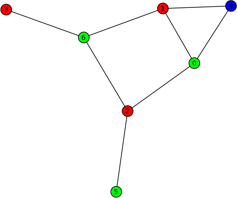
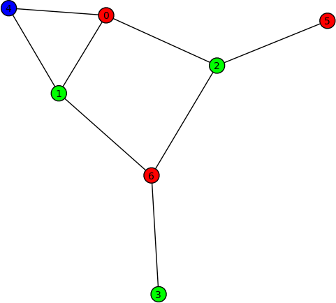
| * FIXME: summarize #5913 | * Graph colouring (Robert Miller) -- New method {{{coloring()}}} of the class {{{sage.graphs.graph.Graph}}} for obtaining the first (optimal) coloring found on a graph. Here are some examples on using this new method: {{{ sage: G = Graph("Fooba") sage: P = G.coloring() sage: G.plot(partition=P) sage: H = G.coloring(hex_colors=True) sage: G.plot(vertex_colors=H) }}} {{attachment:graph-colour-1.png}} {{attachment:graph-colour-2.png}} * FIXME: summarize #6066 * FIXME: summarize #3932 * FIXME: summarize #5940 * FIXME: summarize #6086 |
| Line 70: | Line 175: |
| * FIXME: summarize #5664 * FIXME: summarize #5844 |
* Improved efficiency of {{{is_subgroup}}} (Simon King) -- Testing whether a group is a subgroup of another group is now up to 2x faster than previously. The following timing statistics were obtained using the machine sage.math: {{{ # BEFORE sage: G = SymmetricGroup(7) sage: H = SymmetricGroup(6) sage: %time H.is_subgroup(G) CPU times: user 4.12 s, sys: 0.53 s, total: 4.65 s Wall time: 5.51 s True sage: %timeit H.is_subgroup(G) 10000 loops, best of 3: 118 µs per loop # AFTER sage: G = SymmetricGroup(7) sage: H = SymmetricGroup(6) sage: %time H.is_subgroup(G) CPU times: user 0.00 s, sys: 0.00 s, total: 0.00 s Wall time: 0.00 s True sage: %timeit H.is_subgroup(G) 10000 loops, best of 3: 56.3 µs per loop }}} |
| Line 78: | Line 206: |
| * Viewing Sage objects with a PDF viewer (INSERT CREDIT) -- Implements the option {{{viewer="pdf"}}} for the command {{{view()}}} so that one can invoke this command in the form {{{view(object, viewer="pdf")}}} in order to view {{{object}}} using a PDF viewer. Typical uses of this new optional argument include: | * Viewing Sage objects with a PDF viewer (Nicolas Thiery) -- Implements the option {{{viewer="pdf"}}} for the command {{{view()}}} so that one can invoke this command in the form {{{view(object, viewer="pdf")}}} in order to view {{{object}}} using a PDF viewer. Typical uses of this new optional argument include: |
| Line 83: | Line 211: |
| * FIXME: summarize #6039 | * Change name of Pari's {{{sum}}} function when imported (Craig Citro) -- When Pari's {{{sum}}} function is imported, it is renamed to {{{pari_sum}}} in order to avoid conflict Python's {{{sum}}} function. |
| Line 88: | Line 216: |
| * FIXME: summarize #5974 | * Improved performance for the generic {{{linear_combination_of_rows}}} and {{{linear_combination_of_columns}}} functions for matrices (William Stein) -- The speed-up for the generic functions {{{linear_combination_of_rows}}} and {{{linear_combination_of_columns}}} is up to 4x. The following timing statistics were obtained using the machine sage.math: {{{ # BEFORE sage: A = random_matrix(QQ, 50) sage: v = [1..50] sage: %timeit A.linear_combination_of_rows(v); 1000 loops, best of 3: 1.99 ms per loop sage: %timeit A.linear_combination_of_columns(v); 1000 loops, best of 3: 1.97 ms per loop # AFTER sage: A = random_matrix(QQ, 50) sage: v = [1..50] sage: %timeit A.linear_combination_of_rows(v); 1000 loops, best of 3: 436 µs per loop sage: %timeit A.linear_combination_of_columns(v); 1000 loops, best of 3: 457 µs per loop }}} |
| Line 94: | Line 244: |
| * FIXME: summarize #5554 |
|
| Line 97: | Line 249: |
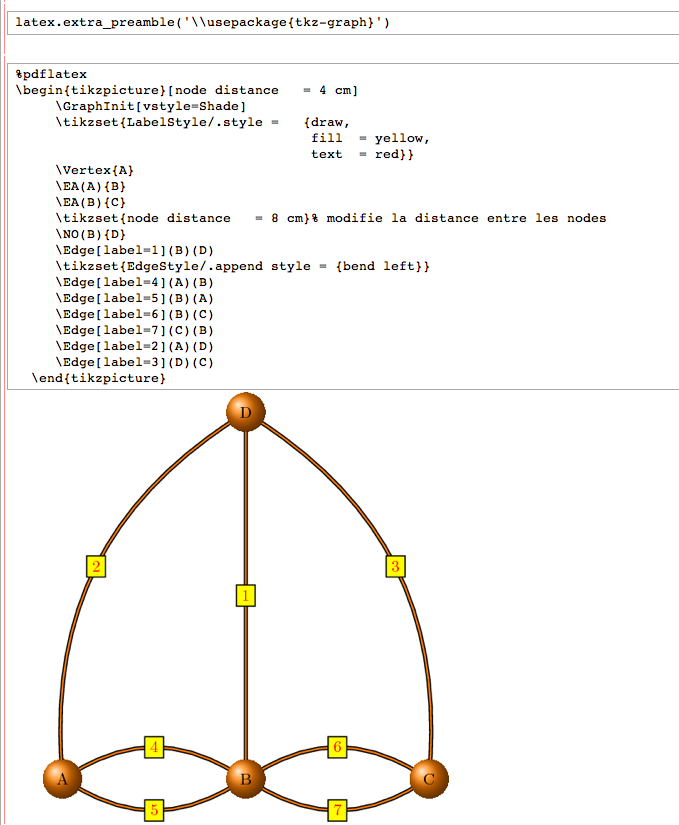
| * FIXME: summarize #6012 | * Allow use of {{{pdflatex}}} instead of {{{latex}}} (John Palmieri) -- One can now use {{{pdflatex}}} instead of {{{latex}}} in two different ways: * Use a {{{%pdflatex}}} cell in a notebook; or * Call {{{latex.pdflatex(True)}}} after which any use of {{{latex}}} (in a {{{%latex}}} cell or using the {{{view}}} command) will use {{{pdflatex}}}. One visually appealing aspect of this is that if you have the most recent version of [[http://pgf.sourceforge.net|pgf]] installed, as well as the {{{tkz-graph}}} package, you can produce images like the following: {{attachment:pgf-graph.png}} * FIXME: summarize #5783 |
| Line 130: | Line 289: |
| * FIXME: summarize #6059 * FIXME: summarize #6064 |
|
| Line 153: | Line 316: |
| * FIXME: summarize #5236 |
|
| Line 157: | Line 322: |
| * FIXME: summarize #6037 |
|
| Line 160: | Line 328: |
| * FIXME: summarize #5777 |
|
| Line 162: | Line 333: |
| * FIXME: summarize #5889 | * Random simplicial complexes (John Palmieri) -- New method {{{RandomComplex()}}} in the module {{{sage/homology/examples.py}}} for producing a random {{{d}}}-dimensional simplicial complex on {{{n}}} vertices. Here's an example: {{{ sage: simplicial_complexes.RandomComplex(6,12) Simplicial complex with vertex set (0, 1, 2, 3, 4, 5, 6, 7) and facets {(0, 1, 2, 3, 4, 5, 6, 7)} }}} |
Sage 4.0 Release Tour
Sage 4.0 was released on FIXME. For the official, comprehensive release note, please refer to sage-4.0.txt. A nicely formatted version of this release tour can be found at FIXME. The following points are some of the foci of this release:
Algebra
Deprecate the order() method on elements of rings (John Palmieri) -- The method order() of the class sage.structure.element.RingElement is now deprecated and will be removed in a future release. For additive or multiplicative order, use the additive_order or multiplicative_order method respectively.
- FIXME: summarize #6052
Algebraic Geometry
Various invariants for genus 2 hyperelliptic curves (Nick Alexander) -- The following invariants for genus 2 hyperelliptic curves are implemented in the module sage/schemes/hyperelliptic_curves/hyperelliptic_g2_generic.py:
- the Clebsch invariants
- the Igusa-Clebsch invariants
- the absolute Igusa invariants
Basic Arithmetic
- FIXME: summarize #6036
- FIXME: summarize #6080
Build
Calculus
Coercion
Combinatorics
ASCII art output for Dynkin diagrams (Dan Bump) -- Support for ASCII art representation of Dynkin diagrams of a finite Cartan type. Here are some examples:
sage: DynkinDiagram("E6")

        O 2
        |
        |
O---O---O---O---O
1   3   4   5   6
E6
sage: DynkinDiagram(['E',6,1])

        O 0
        |
        |
        O 2
        |
        |
O---O---O---O---O
1   3   4   5   6
E6~
Commutative Algebra
Improved performance for SR (Martin Albrecht) -- The speed-up gain for SR is up to 6x. The following timing statistics were obtained using the machine sage.math:
# BEFORE

sage: sr = mq.SR(4, 4, 4, 8, gf2=True, polybori=True, allow_zero_inversions=True)
sage: %time F,s = sr.polynomial_system()
CPU times: user 21.65 s, sys: 0.03 s, total: 21.68 s
Wall time: 21.83 s


# AFTER

sage: sr = mq.SR(4, 4, 4, 8, gf2=True, polybori=True, allow_zero_inversions=True)
sage: %time F,s = sr.polynomial_system()
CPU times: user 3.61 s, sys: 0.06 s, total: 3.67 s
Wall time: 3.67 s
Symmetric Groebner bases and infinitely generated polynomial rings (Simon King, Mike Hansen) -- The new modules sage/rings/polynomial/infinite_polynomial_element.py and sage/rings/polynomial/infinite_polynomial_ring.py support computation in polynomial rings with a countably infinite number of variables. Here are some examples for working with these new modules:
sage: from sage.rings.polynomial.infinite_polynomial_element import InfinitePolynomial
sage: X.<x> = InfinitePolynomialRing(QQ)
sage: a = InfinitePolynomial(X, "(x1 + x2)^2"); a
x2^2 + 2*x2*x1 + x1^2
sage: p = a.polynomial()
sage: b = InfinitePolynomial(X, a.polynomial())
sage: a == b
True
sage: InfinitePolynomial(X, int(1))
1
sage: InfinitePolynomial(X, 1)
1
sage: Y.<x,y> = InfinitePolynomialRing(GF(2), implementation="sparse")
sage: InfinitePolynomial(Y, a)
x2^2 + x1^2

sage: X.<x,y> = InfinitePolynomialRing(QQ, implementation="sparse")
sage: A.<a,b> = InfinitePolynomialRing(QQ, order="deglex")
sage: f = x[5] + 2; f
x5 + 2
sage: g = 3*y[1]; g
3*y1
sage: g._p.parent()
Univariate Polynomial Ring in y1 over Rational Field
sage: f2 = a[5] + 2; f2
a5 + 2
sage: g2 = 3*b[1]; g2
3*b1
sage: A.polynomial_ring()
Multivariate Polynomial Ring in b5, b4, b3, b2, b1, b0, a5, a4, a3, a2, a1, a0 over Rational Field
sage: f + g
3*y1 + x5 + 2
sage: p = x[10]^2 * (f + g); p
3*y1*x10^2 + x10^2*x5 + 2*x10^2
Furthermore, the new module sage/rings/polynomial/symmetric_ideal.py supports ideals of polynomial rings in a countably infinite number of variables that are invariant under variable permuation. Symmetric reduction of infinite polynomials is provided by the new module sage/rings/polynomial/symmetric_reduction.pyx.
Distribution
Doctest
Documentation
Geometry
Graph Theory
Graph colouring (Robert Miller) -- New method coloring() of the class sage.graphs.graph.Graph for obtaining the first (optimal) coloring found on a graph. Here are some examples on using this new method:
sage: G = Graph("Fooba")
sage: P = G.coloring()
sage: G.plot(partition=P)
sage: H = G.coloring(hex_colors=True)
sage: G.plot(vertex_colors=H)


- FIXME: summarize #6066
- FIXME: summarize #3932
- FIXME: summarize #5940
- FIXME: summarize #6086
Graphics
- FIXME: summarize #5249
Group Theory
Improved efficiency of is_subgroup (Simon King) -- Testing whether a group is a subgroup of another group is now up to 2x faster than previously. The following timing statistics were obtained using the machine sage.math:
# BEFORE

sage: G = SymmetricGroup(7)
sage: H = SymmetricGroup(6)
sage: %time H.is_subgroup(G)
CPU times: user 4.12 s, sys: 0.53 s, total: 4.65 s
Wall time: 5.51 s
True
sage: %timeit H.is_subgroup(G)
10000 loops, best of 3: 118 µs per loop


# AFTER

sage: G = SymmetricGroup(7)
sage: H = SymmetricGroup(6)
sage: %time H.is_subgroup(G)
CPU times: user 0.00 s, sys: 0.00 s, total: 0.00 s
Wall time: 0.00 s
True
sage: %timeit H.is_subgroup(G)
10000 loops, best of 3: 56.3 µs per loop
Interfaces
Viewing Sage objects with a PDF viewer (Nicolas Thiery) -- Implements the option viewer="pdf" for the command view() so that one can invoke this command in the form view(object, viewer="pdf") in order to view object using a PDF viewer. Typical uses of this new optional argument include:
- You prefer to use a PDF viewer rather than a DVI viewer.
- You want to view LaTeX snippets which are not displayed well in DVI viewers (e.g. graphics produced using tikzpicture).
Change name of Pari's sum function when imported (Craig Citro) -- When Pari's sum function is imported, it is renamed to pari_sum in order to avoid conflict Python's sum function.
Linear Algebra
Improved performance for the generic linear_combination_of_rows and linear_combination_of_columns functions for matrices (William Stein) -- The speed-up for the generic functions linear_combination_of_rows and linear_combination_of_columns is up to 4x. The following timing statistics were obtained using the machine sage.math:
# BEFORE

sage: A = random_matrix(QQ, 50)
sage: v = [1..50]
sage: %timeit A.linear_combination_of_rows(v);
1000 loops, best of 3: 1.99 ms per loop
sage: %timeit A.linear_combination_of_columns(v);
1000 loops, best of 3: 1.97 ms per loop


# AFTER

sage: A = random_matrix(QQ, 50)
sage: v = [1..50]
sage: %timeit A.linear_combination_of_rows(v);
1000 loops, best of 3: 436 µs per loop
sage: %timeit A.linear_combination_of_columns(v);
1000 loops, best of 3: 457 µs per loop
- FIXME: summarize #5557
- FIXME: summarize #5381
- FIXME: summarize #5554
Miscellaneous
Allow use of pdflatex instead of latex (John Palmieri) -- One can now use pdflatex instead of latex in two different ways:
Use a %pdflatex cell in a notebook; or
Call latex.pdflatex(True)
after which any use of latex (in a %latex cell or using the view command) will use pdflatex. One visually appealing aspect of this is that if you have the most recent version of pgf installed, as well as the tkz-graph package, you can produce images like the following:

- FIXME: summarize #5783
Modular Forms
- FIXME: summarize #4337
- FIXME: summarize #4357
- FIXME: summarize #5262
- FIXME: summarize #5792
- FIXME: summarize #5796
- FIXME: summarize #6019
- FIXME: summarize #5924
Notebook
Number Theory
- FIXME: summarize #5250
- FIXME: summarize #6013
- FIXME: summarize #6008
- FIXME: summarize #6004
- FIXME: summarize #6059
- FIXME: summarize #6064
Numerical
Packages
- FIXME: summarize #4223
- FIXME: summarize #6031
- FIXME: summarize #5934
- FIXME: summarize #1338
- FIXME: summarize #6032
- FIXME: summarize #6024
P-adics
- FIXME: summarize #5105
- FIXME: summarize #5236
Quadratic Forms
- FIXME: summarize #6037
Symbolics
- FIXME: summarize #5777
Topology
Random simplicial complexes (John Palmieri) -- New method RandomComplex() in the module sage/homology/examples.py for producing a random d-dimensional simplicial complex on n vertices. Here's an example:
sage: simplicial_complexes.RandomComplex(6,12)
Simplicial complex with vertex set (0, 1, 2, 3, 4, 5, 6, 7) and facets {(0, 1, 2, 3, 4, 5, 6, 7)}
User Interface
