|
⇤ ← Revision 1 as of 2010-02-27 01:45:03
Size: 5552
Comment:
|
Size: 5512
Comment:
|
| Deletions are marked like this. | Additions are marked like this. |
| Line 1: | Line 1: |
| == Animations drawn by Sage == |
|
| Line 7: | Line 5: |
| === The witch of Maria Agnesi === | == The witch of Maria Agnesi == |
| Line 46: | Line 44: |
| === A simpler hypotrochoid === | == A simpler hypotrochoid == |
| Line 153: | Line 151: |
| === The Tamer and the Lion by Provencal and Labbe === | == The Tamer and the Lion by Provencal and Labbe == |
These animations were drawn by Sage.
Contents
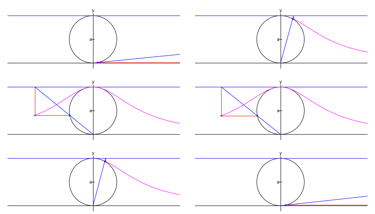
The witch of Maria Agnesi
by Marshall Hampton
xtreme = 4.1
myaxes = line([[-xtreme,0],[xtreme,0]],rgbcolor = (0,0,0))
myaxes = myaxes + line([[0,-1],[0,2.1]],rgbcolor = (0,0,0))
a = 1.0
t = var('t')
npi = RDF(pi)
def agnesi(theta):
    mac = circle((0,a),a,rgbcolor = (0,0,0))
    maL = line([[-xtreme,2*a],[xtreme,2*a]])
    maL2 = line([[0,0],[2*a*cot(theta),2*a]])
    p1 = [2*a*cot(theta),2*a*sin(theta)^2]
    p2 = [2*a*cot(theta)-cot(theta)*(2*a-2*a*sin(theta)^2),2*a*sin(theta)^2]
    maL3 = line([p2,p1,[2*a*cot(theta),2*a]], rgbcolor = (1,0,0))
    map1 = point(p1)
    map2 = point(p2)
    am = line([[-.05,a],[.05,a]], rgbcolor = (0,0,0))
    at = text('a',[-.1,a], rgbcolor = (0,0,0))
    yt = text('y',[0,2.2], rgbcolor = (0,0,0))
    xt = text('x',[xtreme + .1,-.1], rgbcolor = (0,0,0))
    matext = at+yt+xt
    ma = mac+myaxes+maL+am+matext+maL2+map1+maL3+map2
    return ma

def witchy(theta):
    ma = agnesi(theta)
    agplot = parametric_plot([2*a*cot(t),2*a*sin(t)^2],[t,.001,theta], rgbcolor = (1,0,1))
    return ma+agplot

a2 = animate([witchy(i) for i in srange(.1,npi-.1,npi/60)]+[witchy(i) for i in srange(npi-.1,.1,-npi/60)], xmin = -3, xmax = 3, ymin = 0, ymax = 2.3, figsize = [6,2.3], axes = False)

a2.show()

A simpler hypotrochoid
The following animates a hypotrochoid much to the same effect as the previous script, but much more concisely.
import operator

# The colors for various elements of the plot:
class color:
    stylus = (1, 0, 0)
    outer  = (.8, .8, .8)
    inner  = (0, 0, 1)
    plot   = (0, 0, 0)
    center = (0, 0, 0)
    tip    = (1, 0, 0)
# and the corresponding line weights:
class weight:
    stylus = 1
    outer  = 1
    inner  = 1
    plot   = 1
    center = 5
    tip    = 5

scale = 1            # The scale of the image
animation_delay = .1 # The delay between frames, in seconds

# Starting and ending t values
t_i = 0
t_f = 2*pi
# The t values of the animation frames
tvals = srange(t_i, t_f, (t_f-t_i)/60)

r_o = 8 # Outer circle radius
r_i = 2 # Inner circle radius
r_s = 3 # Stylus radius

# Coordinates of the center of the inner circle
x_c = lambda t: (r_o - r_i)*cos(t)
y_c = lambda t: (r_o - r_i)*sin(t)

# Parametric coordinates for the plot
x = lambda t: x_c(t) + r_s*cos(t*(r_o/r_i))
y = lambda t: y_c(t) - r_s*sin(t*(r_o/r_i))

# Maximum x and y values of the plot
x_max = r_o - r_i + r_s
y_max = find_maximum_on_interval(y, t_i, t_f)[0]

# The plots of the individual elements. Order is important; plots
# are stacked from bottom to top as they appear.
elements = (
    # The outer circle
    lambda t_f: circle((0, 0),               r_o, rgbcolor=color.outer, thickness=weight.outer),
    # The plot itself
    lambda t_f: parametric_plot((x, y), t_i, t_f, rgbcolor=color.plot,  thickness=weight.plot),
    # The inner circle
    lambda t_f: circle((x_c(t_f), y_c(t_f)), r_i, rgbcolor=color.inner, thickness=weight.inner),
    # The inner circle's center
    lambda t_f: point((x_c(t_f), y_c(t_f)),       rgbcolor=color.center,pointsize=weight.center),
    # The stylus
    lambda t_f: line([(x_c(t_f), y_c(t_f)), (x(t_f), y(t_f))], rgbcolor=color.stylus, thickness=weight.stylus),
    # The stylus' tip
    lambda t_f: point((x_c(t_f), y_c(t_f)),       rgbcolor=color.tip,   pointsize=weight.tip),
)

# Create the plots and animate them. The animate function renders an
# animated gif from the frames provided as its first argument.
# Though avid python programmers will find the syntax clear, an
# explanation is provided for novices.
animation = animate([sum(f(t) for f in elements)
                     for t in tvals],
                    xmin=-x_max, xmax=x_max,
                    ymin=-y_max, ymax=y_max,
                    figsize=(x_max*scale, y_max*scale * y_max/x_max))

animation.show(delay=animation_delay)

# The previous could be expressed more pedagogically as follows:
#
#   Evaluate each function in the elements array for the provided t
#   value:
#
#     plots = lambda t: f(t) for f in elements
#
#   Join a group of plots together to form a single plot:
#
#     def join_plots(plots):
#         result = plots[0]
#         for plot in plots[1:]:
#             result += plot
#         return result
#
#   or
#
#     join_plots = sum
#
#   Create an array of plots, one for each provided t value:
#
#     frames = [join_plots(plots(t)) for t in tvals]
#
#   Finally, animate the frames:
#
#     animation = animate(frames)
The Tamer and the Lion by Provencal and Labbe
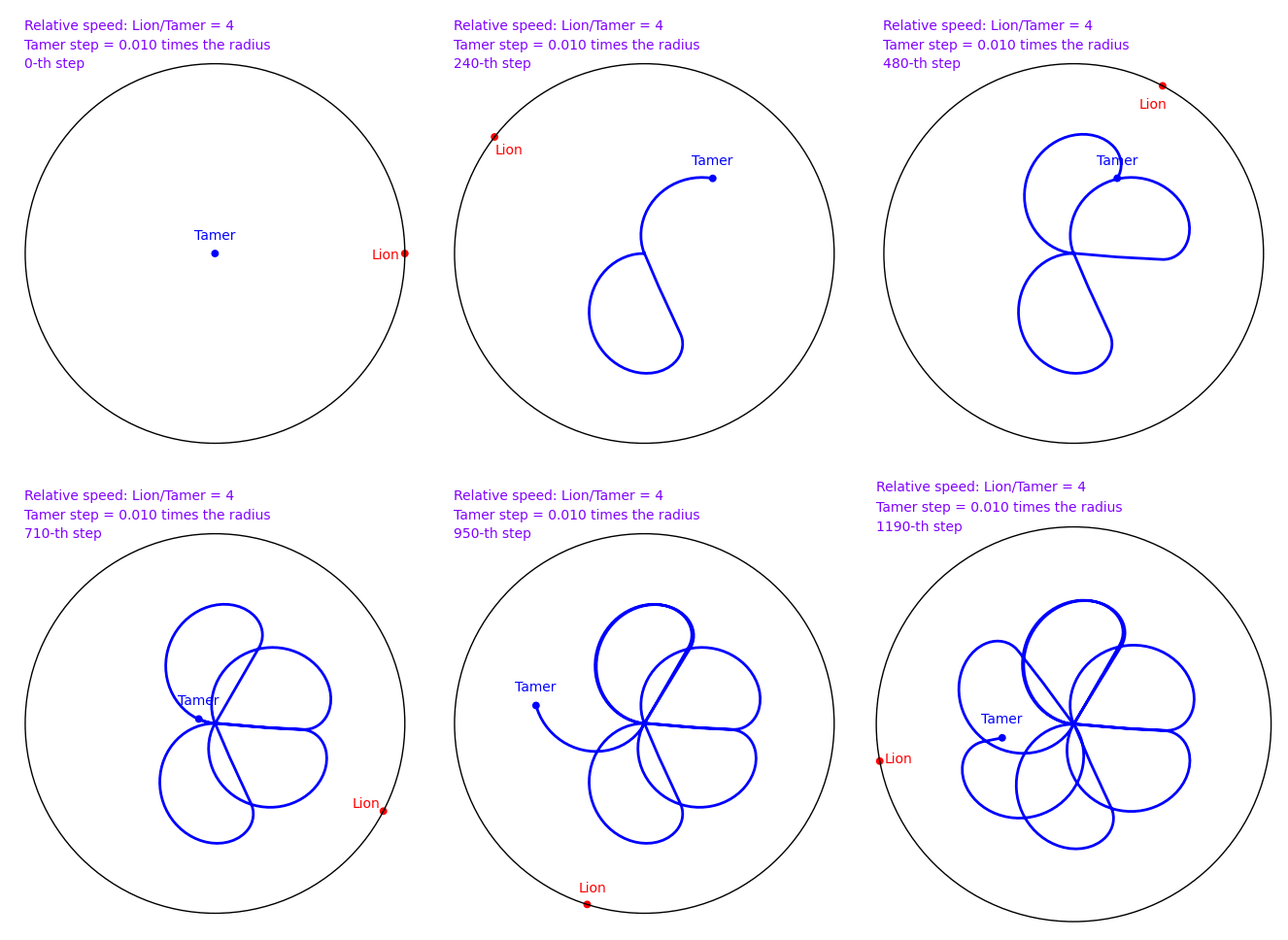
A tamer wants to escape within a circle without being eaten by a lion who lives on the circle. The speed of the lion is 4 times that of the tamer. How can the tamer escape? There is a nice and clever solution in 2d, but does the naive solution where the tamer always moves oppositely to the lion works? In November 2009, Sage and a small script written by Xavier Provençal and Sébastien Labbé in Montpellier answers the question.

To create the above animation, download tamer.sage and type
sage: load tamer.sage
sage: l = range(0,1200,10)
sage: a = anime(l)
sage: a
Animation with 120 frames
sage: show(a)
