|
Size: 22054
Comment: new animations section
|
Size: 25009
Comment: Added: Pencil of conics
|
| Deletions are marked like this. | Additions are marked like this. |
| Line 1: | Line 1: |
| These animations were drawn by [[http://www.sagemath.org|Sage]]. | This page contains animations drawn using [[http://www.sagemath.org|Sage]]. One can create an animation (.gif) in Sage from a list of graphics objects using the {{{animate}}} command. Currently, to export an animation in .gif format, you might need to install the [[http://www.imagemagick.org|ImageMagick]] command line tools package (the ``convert`` command). See the documentation for more information: {{{ sage: animate? }}} |
| Line 479: | Line 484: |
=== The Towers of Hanoi === {{attachment:hanoi.gif}} by Pablo Angulo {{{#!python numbers=off def plot_towers(towers): '''Returns a plot of the towers of Hanoi Uses matrix_plot ''' K=max(max(l) for l in towers if l)+1 M=matrix(ZZ,K,6*K+7) #first tower for t in range(len(towers[0])): j = t k=towers[0][t]-1 for l in range(K+1-k,K+2+k): M[K-1-j,l]=1 #second tower for t in range(len(towers[1])): j = t k=towers[1][t]-1 for l in range(3*K+3-k,3*K+4+k): M[K-1-j,l]=1 #third tower for t in range(len(towers[2])): j = t k=towers[2][t]-1 for l in range(5*K+5-k,5*K+6+k): M[K-1-j,l]=1 return matrix_plot(M, axes=False) def animate_towers(towers,a=0,b=1,c=2,k=-1): '''Move last k discs from column a into column b Assumes that the last k discs of column a are all smaller than the discs in columns b and c ''' if k==0: return if k==-1: k=len(towers[a]) for t in animate_towers(towers,a,c,b,k-1): yield t disc = towers[a].pop() towers[b].append(disc) yield plot_towers(towers) for t in animate_towers(towers,c,b,a,k-1): yield t towers = (range(4,0,-1),[],[]) initial = plot_towers(towers) frame_list=[initial]+list(animate_towers(towers)) animate(frame_list, axes=False).show(delay=80) }}} === Fibonacci Tiles === {{attachment:fibotile.gif}} by Sébastien Labbé {{{#!python numbers=off sage: path_op = dict(rgbcolor='red', thickness=1) sage: fill_op = dict(rgbcolor='blue', alpha=0.3) sage: options = dict(pathoptions=path_op, filloptions=fill_op, endarrow=False, startpoint=False) sage: G = [words.fibonacci_tile(i).plot(**options) for i in range(7)] sage: a = animate(G) sage: a.show(delay=150) }}} === Pencil of conics === by Pablo Angulo {{attachment:pencil.gif}} {{{ puntos = [(0,0),(0,1),(1,3),(2,1)] K = len(puntos) var('x y') coefs = matrix(QQ, K, 6) for j in range(K): x0, y0 = puntos[j] coefs[j,:] = vector([x0^2, y0^2, x0*y0, x0, y0, 1]) K = coefs.right_kernel() v1 = K.basis()[0] v2 = K.basis()[1] graficas = [] for t in srange(0,2*pi,0.3): c1, c2 = sin(t), cos(t) a,b,c,d,e,f = c1*v1 + c2*v2 curva = a*x^2 + b*y^2 + c*x*y + d*x + e*y + f graficas.append( point2d(puntos,color=(1,0,0),pointsize=30) + implicit_plot(curva,(x,-1,4),(y,-1,4)) ) a = animate(graficas) a.show(delay=10) }}} |
This page contains animations drawn using Sage. One can create an animation (.gif) in Sage from a list of graphics objects using the animate command. Currently, to export an animation in .gif format, you might need to install the ImageMagick command line tools package (the convert command). See the documentation for more information:
sage: animate?
Contents
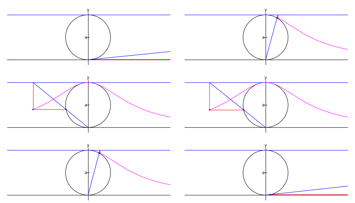
The witch of Maria Agnesi

by Marshall Hampton
xtreme = 4.1
myaxes = line([[-xtreme,0],[xtreme,0]],rgbcolor = (0,0,0))
myaxes = myaxes + line([[0,-1],[0,2.1]],rgbcolor = (0,0,0))
a = 1.0
t = var('t')
npi = RDF(pi)
def agnesi(theta):
    mac = circle((0,a),a,rgbcolor = (0,0,0))
    maL = line([[-xtreme,2*a],[xtreme,2*a]])
    maL2 = line([[0,0],[2*a*cot(theta),2*a]])
    p1 = [2*a*cot(theta),2*a*sin(theta)^2]
    p2 = [2*a*cot(theta)-cot(theta)*(2*a-2*a*sin(theta)^2),2*a*sin(theta)^2]
    maL3 = line([p2,p1,[2*a*cot(theta),2*a]], rgbcolor = (1,0,0))
    map1 = point(p1)
    map2 = point(p2)
    am = line([[-.05,a],[.05,a]], rgbcolor = (0,0,0))
    at = text('a',[-.1,a], rgbcolor = (0,0,0))
    yt = text('y',[0,2.2], rgbcolor = (0,0,0))
    xt = text('x',[xtreme + .1,-.1], rgbcolor = (0,0,0))
    matext = at+yt+xt
    ma = mac+myaxes+maL+am+matext+maL2+map1+maL3+map2
    return ma

def witchy(theta):
    ma = agnesi(theta)
    agplot = parametric_plot([2*a*cot(t),2*a*sin(t)^2],[t,.001,theta], rgbcolor = (1,0,1))
    return ma+agplot

a2 = animate([witchy(i) for i in srange(.1,npi-.1,npi/60)]+[witchy(i) for i in srange(npi-.1,.1,-npi/60)], xmin = -3, xmax = 3, ymin = 0, ymax = 2.3, figsize = [6,2.3], axes = False)

a2.show()
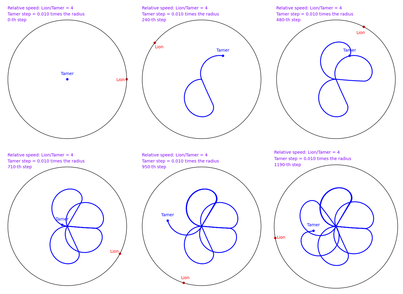
The Tamer and the Lion by Provencal and Labbe
A tamer wants to escape within a circle without being eaten by a lion who lives on the circle. The speed of the lion is 4 times that of the tamer. How can the tamer escape? There is a nice and clever solution in 2d, but does the naive solution where the tamer always moves oppositely to the lion works? In November 2009, Sage and a small script written by Xavier Provençal and Sébastien Labbé in Montpellier answers the question.

To create the above animation, download tamer.sage and type
sage: load tamer.sage
sage: l = range(0,1200,10)
sage: a = anime(l)
sage: a
Animation with 120 frames
sage: show(a)
A hypotrochoid animation by Dean Moore
Hypotrochoid. Written by Dean Moore, February 2008

- Inspiration:
But a Sage newbie & out to do projects & learn more, one day I was surfing Wikipedia and hit < http://en.wikipedia.org/wiki/Hypotrochoid >, saw the animated graph, and thought, ... "I bet I can make Sage do that." Never one to back from a challenge, I did it. A few mistakes & wrong turns, at times some strong language & threatening the computer with violence, a few questions to Sage support groups, but, I finally pounded out code that worked. I named it "Hypotrochoid," as animating this was the original inspiration, but the code easily animates other graphs. What this program does: This program animates (not just "draws," but "animates") graphs of several relations, the hypotrochoid, the hypocycloid, the limacon (or "limacon of Pascal"; Sage doesn't like the French character in the original), the cardioid, the epitrochoid, and the epicycloid. The parametric equations that define a hypotrochoid follow; the parameter
is *t*; for hypotrochoid we have R, r, d > 0, R > r > 0:
 x-coordinate: x = (R - r)*cos(t) + d*cos(((R - r)/r)*t)
 y-coordinate: y = (R - r)*sin(t) - d*sin(((R - r)/r)*t)
- For a epitrochoid, the equations are:
 x = (R + r)*cos(t) - d*cos(((R + r)/r)*t)
 y = (R + r)*sin(t) - d*sin(((R + r)/r)*t)
- The parametric equations are important in computing the period of the relation (below). These parametric equations live all over the Internet; Wikipedia has:
* for the hypochotroid: < http://en.wikipedia.org/wiki/Hypotrochoid >.
See also < http://linuxgazette.net/133/luana.html >
* For the epitrochoid, see < http://en.wikipedia.org/wiki/Epitrochoid >.
- * For the Limacon (Sage completely choked and spewed error messages on the
< http://en.wikipedia.org/wiki/Lima%C3%A7on >.
* For the cardioid, see < http://en.wikipedia.org/wiki/Cardioid >.
* For the epitrochoid, see < < http://en.wikipedia.org/wiki/Epitrochoid >
* For the hypocycloid, see < http://en.wikipedia.org/wiki/Hypocycloid >
* For the Deltoid Curve, see < http://en.wikipedia.org/wiki/Deltoid_curve >.
< http://en.wikipedia.org/wiki/Roulette_%28curve%29 > may be easily animated with this program, as follows: 1) The epitrochoid (use the negative of "small" radius *r*, easy, puts
- rotating circle on the outside.
2) The hypocycloid, by setting 0 < r < R, d = r. 3) The limacon (or "limacon of Pascal"; Sage doesn't like the French
character in the original), use r < 0, R = abs(r).
4) The epicycloid, use r < 0 (put rotating circle on outside), d = r
5) The cardioid, r < 0 d = r
To draw different graphs, vary that parameters *R* (fixed circle's radius), *r* (rotating circle's radius), and *d* (length of "bar" from rotating circle), below; other parameters may be tweaked at will.
Of some note, the *epitrochoid* is the "epicycle" curve of Ptolemaic system astronomy; one project is to animate some of the Ptolemaic system, but this is for the future.
Program commences:
#*****************************************************************************
#       Copyright (C) 2007 Dean Moore < dino@boulder.net >
#
#  Distributed under the terms of the GNU General Public License (GPL)
#                  http://www.gnu.org/licenses/
#*****************************************************************************
# Parameters that define the image:

R = 5   # Fixed circle's radius.
r = 3   # Rotating circle's radius, rotates about fixed circle's radius; make
        # this negative to place rotating circle on outside.
d = 5   # Length of the "bar" extending from the center of the rotating circle.

step = 0.025    # Size of "step" in below loops; the smaller the step, the more
                # "frames" in the final "movie" & the better the image, but the
                # slower the program runs -- and the more bytes to the image.

figuresize = 4  # A constant, regulates size of final picture

delayBetweenImages = 0 # A constant, delay between images in final "movie."

colorOfFixedCircle    = (0, 0, 1) # Colors of final image,
colorOfRotatingCircle = (0, 1, 0) # all described by
colorOfCenterPoint    = (0, 0, 0) # names.
colorOfBar            = (0, 0, 0)
colorOfCurve          = (1, 0, 0)

thicknessOfFixedCircle            =  1   # Thickness of "fixed" circle that never moves.
thicknessOfRotatingCircle         =  1   # Thickness of circle that rotates.
thicknessOfCenterOfRotatingCircle = 15   # Size of small circle's center.
thicknessOfBar                    =  1   # Thickness of "bar" from rotating circle.
penSize                           = 10   # Size of "pen" at end of the "bar."
thicknessOfCurve                  =  0.5 # Thickness of final curve, really a lot of line segments.

# End of parameters user can realistically vary.

origin = (0, 0) # Maybe irrelevant, but NO MAGIC NUMBERS!!  See
                # < http://en.wikipedia.org/wiki/Magic_number_(programming) >.
                # Comes from my days as a C/C++ programmer.

# Graphic parameters, defined here:

L = Graphics() # Graphics for the curve -- really a lot of segments of straight
               # lines.  If the image looks choppy, drop variable *step* above.

v = []         # Holds the curve from *L*, later converted to variable *curve*.

# More parameters, all of which are defined by earlier parameters:

rDiff = (R-r)              # The rotating circle may exceed fixed circle;
                           # values may be negative, so we may have a
                           # negative value.  We use this so much, we give
                           # it a name.

sizeOfGraph = max(R, abs(r) + abs(d), abs(R) - (r) + abs(d)) # Big as it can get -- may be
                                                             # a liberal estimate.

circle2PI = (abs(rDiff)/r).denom() # Number of rotations about 2*pi.  It
                                   # takes a bit of thought, but see the above
                                   # parametric equations.  An example is best:
                                   # picture R=8, r=6.  We have
                                   # (rDiff)/r = (8-6)/6 = 2/6 = 1/3, reduced. For
                                   # the argument *((rDiff)/r)t* to get back to 2*pi
                                   # (i.e., zero) in cos(((R - r)/r)t) & sin(((R - r)/r)t),
                                   # we need to go 2*(3*pi).  A pen & paper & some
                                   # scribbling makes this easy, be it this not
                                   # clear.  The *abs* is probably irrelevant.

limit =  ceil(2*circle2PI/step)    # Loop about circle this many times, by *step*.
                                   # Parameter *circle2PI* never is again used.  Factor
                                   # of 2 is unavoidable, circle 2*pi; see below loops.
First: I use the same trig functions, over an over again. Why re-invent the wheel & waste computer time? Put the needed trig functions in arrays & "recycle" them as needed.
sin1 = [ 0 for i in range(limit) ] # First
sin2 = [ 0 for i in range(limit) ] # define
cos1 = [ 0 for i in range(limit) ] # arrays, ...
cos2 = [ 0 for i in range(limit) ]

increment = 0 # Adding a bunch of numbers is more efficient than multiplying
              # *i*pi*step, but it is a trivial difference.

multiplier = pi*rDiff/r # Efficiency!  Don't repeat the same math
                        # countless times.

for i in srange(limit): # Note above definition of parameter *limit*, the
                        # factor of 2, and the below trig functions.  All
                        # this program's loops go *limit*.

    sin1[i] = sin(increment*pi)         # Now fill
    cos1[i] = cos(increment*pi)         # arrays
    sin2[i] = sin(increment*multiplier) # with our trig
    cos2[i] = cos(increment*multiplier) # functions.

    increment += step                   # End *i*-loop.
The next are described by names, but a few notes:
- * The parameter *fixedCircle* is merely a circle of radius *R* centered at the origin.
I animated it, as that makes it appear in all frames. It never moves.
- * The parameter *rotatingCircle* is more computation-intense. It's center is on the
circle at *rDiff* from the edge of the fixed circle; its radius is *r*, and it rotates about the fixed circle a total of *circle2PI* times. Find any internet reference on these curves to see it.
- * The parameter *centerPoints* is solely to make the rotating circle look nicer,
a clear center.
- * The parameter *bar* is the "bar" extending from the center of the rotating circle,
that follows its rotation around the fixed circle. It always emanates from the same center as *fixedCircle*, -- see *fixedCircle* documentation, above -- and its terminal point comes from the parametric equation of a hypotrochoid (top).
- * The parameter *pointAtPen* makes a point where the end of the bar draws the figure,
of the same color as the final curve. Note it is at the same point as the terminal point of the "bar."
fixedCircle     = animate([circle(origin, R,          # Centered at origin, radius *R*.
                           rgbcolor=colorOfFixedCircle,
                           thickness = thicknessOfFixedCircle)
                           for i in srange(limit)            # Animating loop.
                          ],
                           xmin=-sizeOfGraph, ymin=-sizeOfGraph,
                           xmax= sizeOfGraph, ymax= sizeOfGraph,
                           figsize=[figuresize, figuresize])

rotatingCircle  = animate([circle((rDiff*cos1[i],rDiff*sin1[i]), r, # Note center, radius *r*
                           thickness = thicknessOfRotatingCircle,
                           rgbcolor=colorOfRotatingCircle)
                           for i in srange(limit)        # Animating loop
                          ],
                           xmin=-sizeOfGraph, ymin=-sizeOfGraph,
                           xmax= sizeOfGraph, ymax= sizeOfGraph,
                           figsize=[figuresize,figuresize])

centerPoints    = animate([point((rDiff*cos1[i],rDiff*sin1[i]), # Center of *fixedCircle*.
                           rgbcolor=colorOfCenterPoint,
                           pointsize=thicknessOfCenterOfRotatingCircle)
                           for i in srange(limit)                      # Animating loop
                          ],
                           xmin=-sizeOfGraph, ymin=-sizeOfGraph,
                           xmax= sizeOfGraph, ymax= sizeOfGraph,
                           figsize=[figuresize,figuresize])

bar             = animate(line([(rDiff*cos1[i], rDiff*sin1[i]), # Starts here, and ...
                                (d*cos2[i] + rDiff*cos1[i],     # Ends at
                                  rDiff*sin1[i] - d*sin2[i])    # this point.
                               ],
                           thickness = thicknessOfBar,
                           rgbcolor=colorOfBar)
                           for i in srange(limit))               # Animating loop

pointAtPen      = animate([point((d*cos2[i]+rDiff*cos1[i],     # End of pen, same x & y
                                 (rDiff)*sin1[i] - d*sin2[i]), # coordinates as endpoints of *bar*
                           rgbcolor=colorOfCurve,
                           pointsize=penSize)
                           for i in srange(limit)                   # Animating loop
                           ],
                           xmin=-sizeOfGraph, ymin=-sizeOfGraph,
                           xmax= sizeOfGraph, ymax= sizeOfGraph,
                           figsize=[figuresize,figuresize])

# Prepare to draw the curve; we use four "important" variables: x0, x1, y0 & y1;
# the line segment goes from (x0, y0) to (x1, y1):

x0 = rDiff + d     # Initial values of these variables; bumped up at bottom
                   # of next loop -- see a graph or look at parametric equations
                   # at zero to understand why it has this value.

y0 = 0             # The "pen" out the small circle starts at this (x0, y0).

# Now to compute the curve, in the next loop.  Starts at zero, even if
# this seems to make the first a junk computation; otherwise the output
# looks weird:

for i in srange(limit): # Parameter *circle2PI* is number of times we rotate
                        # the "fixed" circle; limit=2*circle2PI; see above
                        # documentation.

    x1 = rDiff*cos1[i] + d*cos2[i]   # Initial, starting point of
                                    # the line; see parametric
                                    # equations.

    y1 = rDiff*sin1[i] - d*sin2[i] # Again, see the parametric
                                  # equation at top.
    # Now make the line:

    L += line([(x0, y0),(x1, y1)], rgbcolor = colorOfCurve , thickness=thicknessOfCurve)

    L.xmin(-sizeOfGraph)  # Some nonsense
    L.ymin(-sizeOfGraph)  # that needs done.
    L.xmax( sizeOfGraph)
    L.ymax( sizeOfGraph)

    x0 = x1 # Bump up these variables, start of
    y0 = y1 # next line segment is end of last.

    v.append(L) # *** End of loop ***
               # Stash curve *L* in the variable *v*.

curve = animate(v) # Animate the curve, and ...

# Show the entire "movie":

(fixedCircle + rotatingCircle + pointAtPen + bar + centerPoints + curve).show(delay=delayBetweenImages)
We've shown the final image; done with program.
A simpler hypotrochoid
The following animates a hypotrochoid much to the same effect as the previous script, but much more concisely.
import operator

# The colors for various elements of the plot:
class color:
    stylus = (1, 0, 0)
    outer  = (.8, .8, .8)
    inner  = (0, 0, 1)
    plot   = (0, 0, 0)
    center = (0, 0, 0)
    tip    = (1, 0, 0)
# and the corresponding line weights:
class weight:
    stylus = 1
    outer  = 1
    inner  = 1
    plot   = 1
    center = 5
    tip    = 5

scale = 1            # The scale of the image
animation_delay = .1 # The delay between frames, in seconds

# Starting and ending t values
t_i = 0
t_f = 2*pi
# The t values of the animation frames
tvals = srange(t_i, t_f, (t_f-t_i)/60)

r_o = 8 # Outer circle radius
r_i = 2 # Inner circle radius
r_s = 3 # Stylus radius

# Coordinates of the center of the inner circle
x_c = lambda t: (r_o - r_i)*cos(t)
y_c = lambda t: (r_o - r_i)*sin(t)

# Parametric coordinates for the plot
x = lambda t: x_c(t) + r_s*cos(t*(r_o/r_i))
y = lambda t: y_c(t) - r_s*sin(t*(r_o/r_i))

# Maximum x and y values of the plot
x_max = r_o - r_i + r_s
y_max = find_maximum_on_interval(y, t_i, t_f)[0]

# The plots of the individual elements. Order is important; plots
# are stacked from bottom to top as they appear.
elements = (
    # The outer circle
    lambda t_f: circle((0, 0),               r_o, rgbcolor=color.outer, thickness=weight.outer),
    # The plot itself
    lambda t_f: parametric_plot((x, y), t_i, t_f, rgbcolor=color.plot,  thickness=weight.plot),
    # The inner circle
    lambda t_f: circle((x_c(t_f), y_c(t_f)), r_i, rgbcolor=color.inner, thickness=weight.inner),
    # The inner circle's center
    lambda t_f: point((x_c(t_f), y_c(t_f)),       rgbcolor=color.center,pointsize=weight.center),
    # The stylus
    lambda t_f: line([(x_c(t_f), y_c(t_f)), (x(t_f), y(t_f))], rgbcolor=color.stylus, thickness=weight.stylus),
    # The stylus' tip
    lambda t_f: point((x_c(t_f), y_c(t_f)),       rgbcolor=color.tip,   pointsize=weight.tip),
)

# Create the plots and animate them. The animate function renders an
# animated gif from the frames provided as its first argument.
# Though avid python programmers will find the syntax clear, an
# explanation is provided for novices.
animation = animate([sum(f(t) for f in elements)
                     for t in tvals],
                    xmin=-x_max, xmax=x_max,
                    ymin=-y_max, ymax=y_max,
                    figsize=(x_max*scale, y_max*scale * y_max/x_max))

animation.show(delay=animation_delay)

# The previous could be expressed more pedagogically as follows:
#
#   Evaluate each function in the elements array for the provided t
#   value:
#
#     plots = lambda t: f(t) for f in elements
#
#   Join a group of plots together to form a single plot:
#
#     def join_plots(plots):
#         result = plots[0]
#         for plot in plots[1:]:
#             result += plot
#         return result
#
#   or
#
#     join_plots = sum
#
#   Create an array of plots, one for each provided t value:
#
#     frames = [join_plots(plots(t)) for t in tvals]
#
#   Finally, animate the frames:
#
#     animation = animate(frames)
The Towers of Hanoi

by Pablo Angulo
def plot_towers(towers):
    '''Returns a plot of the towers of Hanoi

    Uses matrix_plot
    '''
    K=max(max(l) for l in towers if l)+1
    M=matrix(ZZ,K,6*K+7)
    #first tower
    for t in range(len(towers[0])):
        j = t
        k=towers[0][t]-1
        for l in range(K+1-k,K+2+k):
            M[K-1-j,l]=1
    #second tower
    for t in range(len(towers[1])):
        j = t
        k=towers[1][t]-1
        for l in range(3*K+3-k,3*K+4+k):
            M[K-1-j,l]=1
    #third tower
    for t in range(len(towers[2])):
        j = t
        k=towers[2][t]-1
        for l in range(5*K+5-k,5*K+6+k):
            M[K-1-j,l]=1

    return matrix_plot(M, axes=False)

def animate_towers(towers,a=0,b=1,c=2,k=-1):
    '''Move last k discs from column a into column b

    Assumes that the last k discs of column a are all smaller
    than the discs in columns b and c
    '''
    if k==0:  return
    if k==-1: k=len(towers[a])
    for t in animate_towers(towers,a,c,b,k-1):
        yield t
    disc = towers[a].pop()
    towers[b].append(disc)
    yield plot_towers(towers)
    for t in animate_towers(towers,c,b,a,k-1):
        yield t

towers = (range(4,0,-1),[],[])
initial = plot_towers(towers)
frame_list=[initial]+list(animate_towers(towers))
animate(frame_list, axes=False).show(delay=80)
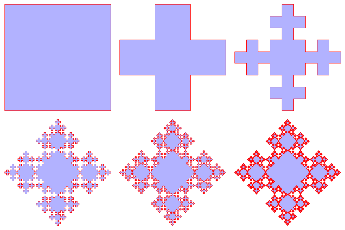
Fibonacci Tiles

by Sébastien Labbé
sage: path_op = dict(rgbcolor='red', thickness=1)
sage: fill_op = dict(rgbcolor='blue', alpha=0.3)
sage: options = dict(pathoptions=path_op, filloptions=fill_op, endarrow=False, startpoint=False)
sage: G = [words.fibonacci_tile(i).plot(**options) for i in range(7)]
sage: a = animate(G)
sage: a.show(delay=150)
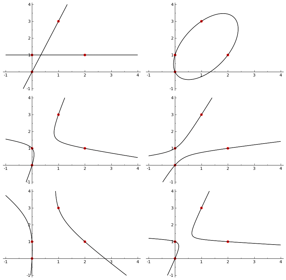
Pencil of conics
by Pablo Angulo 
puntos = [(0,0),(0,1),(1,3),(2,1)]
K = len(puntos)

var('x y')
coefs = matrix(QQ, K, 6)
for j in range(K):
    x0, y0 = puntos[j]
    coefs[j,:] = vector([x0^2, y0^2, x0*y0, x0, y0, 1])

K = coefs.right_kernel()
v1 = K.basis()[0]
v2 = K.basis()[1]

graficas = []
for t in srange(0,2*pi,0.3):
    c1, c2 = sin(t), cos(t)
    a,b,c,d,e,f = c1*v1 + c2*v2
    curva = a*x^2 + b*y^2 + c*x*y + d*x + e*y + f
    graficas.append( point2d(puntos,color=(1,0,0),pointsize=30) +
                     implicit_plot(curva,(x,-1,4),(y,-1,4)) )
a = animate(graficas)

a.show(delay=10)