|
Size: 45695
Comment: minor changes in "coordinate transformations"
|
Size: 57661
Comment: make interacts live.
|
| Deletions are marked like this. | Additions are marked like this. |
| Line 6: | Line 6: |
| Line 9: | Line 10: |
| {{{ | {{{#!sagecell |
| Line 56: | Line 57: |
| {{{ | http://sagenb.org/home/pub/2824/ {{{#!sagecell |
| Line 72: | Line 75: |
| var('x') | |
| Line 79: | Line 84: |
| print "f(c) = %r"%f(z) | print "f(c) = %r"%f(x=z) |
| Line 83: | Line 88: |
| P = plot(f, z-interval, z+interval, rgbcolor='blue') | P = plot(f, (x,z-interval, z+interval), rgbcolor='blue') |
| Line 94: | Line 99: |
| {{{ | http://sagenb.org/home/pub/2823/ {{{#!sagecell |
| Line 101: | Line 108: |
| C = contour_plot(f, (-2,2), (-2,2), plot_points=30, contours=15, cmap=cmap) | C = contour_plot(f, (x,-2,2), (y,-2,2), plot_points=30, contours=15, cmap=cmap) |
| Line 110: | Line 117: |
| {{{ | {{{#!sagecell |
| Line 130: | Line 137: |
| {{{ | {{{#!sagecell |
| Line 158: | Line 165: |
| {{{ | {{{#!sagecell |
| Line 231: | Line 238: |
| {{{ | {{{#!sagecell |
| Line 244: | Line 251: |
| {{{ | {{{#!sagecell |
| Line 342: | Line 349: |
| {{{ | {{{#!sagecell |
| Line 448: | Line 455: |
| {{{ | {{{#!sagecell |
| Line 490: | Line 497: |
| {{{ | {{{#!sagecell |
| Line 513: | Line 520: |
| {{{ | {{{#!sagecell |
| Line 540: | Line 547: |
| {{{ | {{{#!sagecell |
| Line 566: | Line 573: |
| {{{ | {{{#!sagecell |
| Line 581: | Line 588: |
| {{{ | {{{#!sagecell |
| Line 627: | Line 634: |
| {{{ from scipy.special.orthogonal import p_roots |
{{{#!sagecell import scipy import numpy from scipy.special.orthogonal import p_roots, t_roots, u_roots |
| Line 637: | Line 646: |
| 'Chebyshev': {'w': 1/sqrt(1-x**2), 'xmin': -1, 'xmax': 1, 'func': t_roots}, 'Chebyshev2': {'w': sqrt(1-x**2), 'xmin': -1, 'xmax': 1, 'func': u_roots}, 'Trapezoid': {'w': 1, 'xmin': -1, 'xmax': 1, 'func': lambda n: (linspace(-1r,1,n), numpy.array([1.0r]+[2.0r]*(n-2)+[1.0r])*1.0r/n)}, 'Simpson': {'w': 1, 'xmin': -1, 'xmax': 1, 'func': lambda n: (linspace(-1r,1,n), numpy.array([1.0r]+[4.0r,2.0r]*int((n-3.0r)/2.0r)+[4.0r,1.0r])*2.0r/(3.0r*n))}} |
'Chebyshev': {'w': 1/sqrt(1-x**2), 'xmin': -1, 'xmax': 1, 'func': t_roots}, 'Chebyshev2': {'w': sqrt(1-x**2), 'xmin': -1, 'xmax': 1, 'func': u_roots}, 'Trapezoid': {'w': 1, 'xmin': -1, 'xmax': 1, 'func': lambda n: (linspace(-1r,1,n), numpy.array([1.0r]+[2.0r]*(n-2)+[1.0r])*1.0r/n)}, 'Simpson': {'w': 1, 'xmin': -1, 'xmax': 1, 'func': lambda n: (linspace(-1r,1,n), numpy.array([1.0r]+[4.0r,2.0r]*int((n-3.0r)/2.0r)+[4.0r,1.0r])*2.0r/(3.0r*n))}} |
| Line 644: | Line 656: |
| return polygon([(center-width2,0),(center+width2,0),(center+width2,height),(center-width2,height)],**kwds) | return polygon([(center-width2,0), (center+width2,0),(center+width2,height),(center-width2,height)],**kwds) |
| Line 648: | Line 661: |
| def weights(n=slider(1,30,1,default=10),f=input_box(default=3*x+cos(10*x)),show_method=["Legendre", "Chebyshev", "Chebyshev2", "Trapezoid","Simpson"]): | def weights(n=slider(1,30,1,default=10),f=input_box(default=3*x+cos(10*x),type=SR), show_method=["Legendre", "Chebyshev", "Chebyshev2", "Trapezoid","Simpson"]): |
| Line 657: | Line 671: |
| scaled_ff = fast_float(scaled_func) | scaled_ff = fast_float(scaled_func, 'x') |
| Line 665: | Line 679: |
| stems = sum(line([(x,0),(x,scaled_ff(x))],rgbcolor=(1-y,1-y,1-y),thickness=2,markersize=6,alpha=y) for x,y in coords_scaled) points = sum([point([(x,0),(x,scaled_ff(x))],rgbcolor='black',pointsize=30) for x,_ in coords]) |
stems = sum(line([(x,0),(x,scaled_ff(x))],rgbcolor=(1-y,1-y,1-y), thickness=2,markersize=6,alpha=y) for x,y in coords_scaled) points = sum([point([(x,0), (x,scaled_ff(x))],rgbcolor='black',pointsize=30) for x,_ in coords]) |
| Line 671: | Line 687: |
| show(graph,xmin=plot_min,xmax=plot_max) | show(graph,xmin=plot_min,xmax=plot_max,aspect_ratio="auto") |
| Line 679: | Line 695: |
| html("$$\sum_{i=1}^{i=%s}w_i\left(%s\\right)= %s\\approx %s =\int_{-1}^{1}%s \,dx$$"%(n,latex(f.subs(x="x_i")), approximation, integral, latex(scaled_func))) | html("$$\sum_{i=1}^{i=%s}w_i\left(%s\\right)= %s\\approx %s =\int_{-1}^{1}%s \,dx$$"%(n, latex(f), approximation, integral, latex(scaled_func))) |
| Line 692: | Line 709: |
| {{{ | {{{#!sagecell |
| Line 804: | Line 821: |
| {{{ | {{{#!sagecell |
| Line 927: | Line 944: |
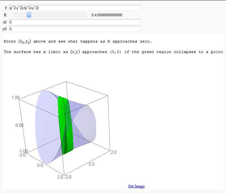
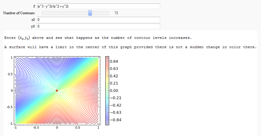
| == Multivariate Limits by Definition == by John Travis http://www.sagenb.org/home/pub/2828/ {{{#!sagecell ## An interactive way to demonstrate limits of multivariate functions of the form z = f(x,y) ## ## John Travis ## Mississippi College ## ## Spring 2011 ## ## An updated version of this worksheet may be available at http://sagenb.mc.edu # Starting point for radius values before collapsing in as R approaches 0. # Functions ought to be "reasonable" within a circular domain of radius R surrounding # the desired (x_0,y_0). Rmax=2 @interact def _(f=input_box(default=(x^3-y^3)/(x^2+y^2)),R=slider(0.1/10,Rmax,1/10,2),x0=(0),y0=(0)): # converting f to cylindrical coordinates. g(r,t) = f(x=r*cos(t)+x0,y=r*sin(t)+y0) # Sage graphing transformation used to see the original surface. cylinder = (r*cos(t)+x0,r*sin(t)+y0,z) surface = plot3d(g,(t,0,2*pi),(r,1/100,Rmax),transformation=cylinder,opacity=0.2) # Regraph the surface for smaller and smaller radii controlled by the slider. limit = plot3d(g,(t,0,2*pi),(r,1/100,R),transformation=cylinder,rgbcolor=(0,1,0)) show(surface+limit) print html('Enter $(x_0 ,y_0 )$ above and see what happens as R approaches zero.') print html('The surface has a limit as $(x,y)$ approaches ('+str(x0)+','+str(y0)+') if the green region collapses to a point') }}} {{attachment:3D_Limit_Defn.png}} {{{#!sagecell ## An interactive way to demonstrate limits of multivariate functions of the form z = f(x,y) ## This one uses contour plots and so will work with functions that have asymptotic behavior. ## ## John Travis ## Mississippi College ## ## Spring 2011 ## # An increasing number of contours for z = f(x,y) are utilized surrounding a desired (x_0,y_0). # A limit can be shown to exist at (x_0,y_0) provided the point stays trapped between adjacent # contour lines as the number of lines increases. If the contours change wildly near the point, # then a limit does not exist. # Looking for two different paths to approach (x_0,y_0) that utilize a different selection of colors # will help locate paths to use that exhibit the absence of a limit. Rmax=2 @interact def _(f=input_box(default=(x^3-y^3)/(x^2+y^2)), N=slider(5,100,1,10,label='Number of Contours'), x0=(0),y0=(0)): print html('Enter $(x_0 ,y_0 )$ above and see what happens as the number of contour levels increases.') print html('A surface will have a limit in the center of this graph provided there is not a sudden change in color there.') surface = contour_plot(f,(x,x0-1,x0+1),(y,y0-1,y0+1),cmap=True,colorbar=True,fill=False,contours=N) limit_point = point((x0,y0),color='red',size=30) show(limit_point+surface)}}} {{attachment:3D_Limit_Defn_Contours.png}} |
|
| Line 931: | Line 1021: |
| {{{ | {{{#!sagecell |
| Line 984: | Line 1074: |
| {{{ %hide %auto |
{{{#!sagecell |
| Line 1045: | Line 1133: |
| {{{ | {{{#!sagecell |
| Line 1083: | Line 1171: |
| {{{ | {{{#!sagecell |
| Line 1116: | Line 1204: |
== Volumes over non-rectangular domains == by John Travis http://www.sagenb.org/home/pub/2829/ {{{#!sagecell ## Graphing surfaces over non-rectangular domains ## John Travis ## Spring 2011 ## ## ## An updated version of this worksheet may be available at http://sagenb.mc.edu ## ## Interact allows the user to input up to two inequality constraints on the ## domain when dealing with functional surfaces ## ## User inputs: ## f = "top" surface with z = f(x,y) ## g = "bottom" surface with z = g(x,y) ## condition1 = a single boundary constraint. It should not include && or | to join two conditions. ## condition2 = another boundary constraint. If there is only one constraint, just enter something true ## or even just an x (or y) in the entry blank. ## ## var('x,y') # f is the top surface # g is the bottom surface global f,g # condition1 and condition2 are the inequality constraints. It would be nice # to have any number of conditions connected by $$ or | global condition1,condition2 @interact def _(f=input_box(default=(1/3)*x^2 + (1/4)*y^2 + 5,label='$f(x)=$'), g=input_box(default=-1*x+0*y,label='$g(x)=$'), condition1=input_box(default= x^2+y^2<8,label='$Constraint_1=$'), condition2=input_box(default=y<sin(3*x),label='$Constraint_2=$'), show_3d=('Stereographic',false), show_vol=('Shade volume',true), dospin = ('Spin?',true), clr = color_selector('#faff00', label='Volume Color', widget='colorpicker', hide_box=True), xx = range_slider(-5, 5, 1, default=(-3,3), label='X Range'), yy = range_slider(-5, 5, 1, default=(-3,3), label='Y Range'), auto_update=false): # This is the top function actually graphed by using NaN outside domain def F(x,y): if condition1(x=x,y=y): if condition2(x=x,y=y): return f(x=x,y=y) else: return -NaN else: return -NaN # This is the bottom function actually graphed by using NaN outside domain def G(x,y): if condition1(x=x,y=y): if condition2(x=x,y=y): return g(x=x,y=y) else: return -NaN else: return -NaN P = Graphics() # The graph of the top and bottom surfaces P_list = [] P_list.append(plot3d(F,(x,xx[0],xx[1]),(y,yy[0],yy[1]),color='blue',opacity=0.9)) P_list.append(plot3d(G,(x,xx[0],xx[1]),(y,yy[0],yy[1]),color='gray',opacity=0.9)) # Interpolate "layers" between the top and bottom if desired if show_vol: ratios = range(10) def H(x,y,r): return (1-r)*F(x=x,y=y)+r*G(x=x,y=y) P_list.extend([ plot3d(lambda x,y: H(x,y,ratios[1]/10),(x,xx[0],xx[1]),(y,yy[0],yy[1]),opacity=0.2,color=clr), plot3d(lambda x,y: H(x,y,ratios[2]/10),(x,xx[0],xx[1]),(y,yy[0],yy[1]),opacity=0.2,color=clr), plot3d(lambda x,y: H(x,y,ratios[3]/10),(x,xx[0],xx[1]),(y,yy[0],yy[1]),opacity=0.2,color=clr), plot3d(lambda x,y: H(x,y,ratios[4]/10),(x,xx[0],xx[1]),(y,yy[0],yy[1]),opacity=0.2,color=clr), plot3d(lambda x,y: H(x,y,ratios[5]/10),(x,xx[0],xx[1]),(y,yy[0],yy[1]),opacity=0.2,color=clr), plot3d(lambda x,y: H(x,y,ratios[6]/10),(x,xx[0],xx[1]),(y,yy[0],yy[1]),opacity=0.2,color=clr), plot3d(lambda x,y: H(x,y,ratios[7]/10),(x,xx[0],xx[1]),(y,yy[0],yy[1]),opacity=0.2,color=clr), plot3d(lambda x,y: H(x,y,ratios[8]/10),(x,xx[0],xx[1]),(y,yy[0],yy[1]),opacity=0.2,color=clr), plot3d(lambda x,y: H(x,y,ratios[9]/10),(x,xx[0],xx[1]),(y,yy[0],yy[1]),opacity=0.2,color=clr) ]) # P = plot3d(lambda x,y: H(x,y,ratio/10),(x,xx[0],xx[1]),(y,yy[0],yy[1]),opacity=0.1) # Now, accumulate all of the graphs into one grouped graph. P = sum(P_list[i] for i in range(len(P_list))) if show_3d: show(P,frame=true,axes=false,xmin=xx[0],xmax=xx[1],ymin=yy[0],ymax=yy[1],stereo='redcyan',figsize=(6,9),viewer='jmol',spin=dospin) else: show(P,frame=true,axes=false,xmin=xx[0],xmax=xx[1],ymin=yy[0],ymax=yy[1],figsize=(6,9),viewer='jmol',spin=dospin) }}} {{attachment:3D_Irregular_Volume.png}} == Lateral Surface Area == by John Travis http://www.sagenb.org/home/pub/2826/ {{{#!sagecell ## Display and compute the area of the lateral surface between two surfaces ## corresponding to the (scalar) line integral ## John Travis ## Spring 2011 var('x,y,t,s') @interact def _(f=input_box(default=6-4*x^2-y^2*2/5,label='$f(x,y) = $'), g=input_box(default=-2+sin(x)+sin(y),label='$g(x,y) = $'), u=input_box(default=cos(t),label='$u(t) = $'), v=input_box(default=2*sin(t),label='$v(t) = $'), a=input_box(default=0,label='$a = $'), b=input_box(default=3*pi/2,label='$b = $'), xx = range_slider(-5, 5, 1, default=(-1,1), label='x view'), yy = range_slider(-5, 5, 1, default=(-2,2), label='y view'), smoother=checkbox(default=false)): ds = sqrt(derivative(u(t),t)^2+derivative(v(t),t)^2) # Set up the integrand to compute the line integral, making all attempts # to simplify the result so that it looks as nice as possible. A = (f(x=u(t),y=v(t))-g(x=u(t),y=v(t)))*ds.simplify_trig().simplify() # It is not expected that Sage can actually perform the line integral calculation. # So, the result displayed may not be a numerical value as expected. # Creating a good but harder example that "works" is desirable. line_integral = integral(A,t,a,b) line_integral_approx = numerical_integral(A,a,b)[0] html(r'<h4 align=center>Lateral Surface Area = $ %s $ </h4>'%latex(line_integral)) html(r'<h4 align=center>Lateral Surface $ \approx $ %s</h2>'%str(line_integral_approx)) # Plot the top function z = f(x,y) that is being integrated. G = plot3d(f,(x,xx[0],xx[1]),(y,yy[0],yy[1]),opacity=0.2) G += plot3d(g,(x,xx[0],xx[1]),(y,yy[0],yy[1]),opacity=0.2) # Add space curves on the surfaces "above" the domain curve (u(t),v(t)) G += parametric_plot3d([u,v,g(x=u(t),y=v(t))],(t,a,b),thickness=2,color='red') G += parametric_plot3d([u,v,f(x=u(t),y=v(t))],(t,a,b),thickness=2,color='red') k=0 if smoother: delw = 0.025 lat_thick = 3 else: delw = 0.10 lat_thick = 10 for w in (a,a+delw,..,b): G += parametric_plot3d([u(w),v(w),s*f(x=u(w),y=v(w))+(1-s)*g(x=u(w),y=v(w))],(s,0,1),thickness=lat_thick,color='yellow',opacity=0.9) show(G,spin=true) }}} {{attachment:Lateral_Surface.png}} |
|
| Line 1118: | Line 1375: |
| {{{ | {{{#!sagecell |
| Line 1132: | Line 1389: |
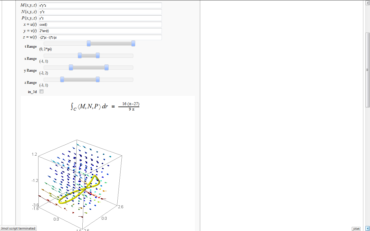
== Line Integrals in 3D Vector Field == by John Travis http://www.sagenb.org/home/pub/2827/ {{{#!sagecell ## This worksheet interactively computes and displays the line integral of a 3D vector field ## over a given smooth curve C ## ## John Travis ## Mississippi College ## 06/16/11 ## ## An updated version of this worksheet may be available at http://sagenb.mc.edu ## var('x,y,z,t,s') @interact def _(M=input_box(default=x*y*z,label="$M(x,y,z)$"), N=input_box(default=-y*z,label="$N(x,y,z)$"), P=input_box(default=z*y,label="$P(x,y,z)$"), u=input_box(default=cos(t),label="$x=u(t)$"), v=input_box(default=2*sin(t),label="$y=v(t)$"), w=input_box(default=t*(t-2*pi)/pi,label="$z=w(t)$"), tt = range_slider(-2*pi, 2*pi, pi/6, default=(0,2*pi), label='t Range'), xx = range_slider(-5, 5, 1, default=(-1,1), label='x Range'), yy = range_slider(-5, 5, 1, default=(-2,2), label='y Range'), zz = range_slider(-5, 5, 1, default=(-3,1), label='z Range'), in_3d=checkbox(true)): # setup the parts and then compute the line integral dr = [derivative(u(t),t),derivative(v(t),t),derivative(w(t),t)] A = (M(x=u(t),y=v(t),z=w(t))*dr[0] +N(x=u(t),y=v(t),z=w(t))*dr[1] +P(x=u(t),y=v(t),z=w(t))*dr[2]) global line_integral line_integral = integral(A(t=t),t,tt[0],tt[1]) html(r'<h2 align=center>$ \int_{C} \left \langle M,N,P \right \rangle dr $ = $ %s $ </h2>'%latex(line_integral)) G = plot_vector_field3d((M,N,P),(x,xx[0],xx[1]),(y,yy[0],yy[1]),(z,zz[0],zz[1]),plot_points=6) G += parametric_plot3d([u,v,w],(t,tt[0],tt[1]),thickness='5',color='yellow') if in_3d: show(G,stereo='redcyan',spin=true) else: show(G,perspective_depth=true) }}} {{attachment:3D_Line_Integral.png}} |
Sage Interactions - Calculus
goto interact main page
Contents
-
Sage Interactions - Calculus
- Root Finding Using Bisection
- Newton's Method
- A contour map and 3d plot of two inverse distance functions
- A simple tangent line grapher
- Numerical integrals with the midpoint rule
- Numerical integrals with various rules
- Some polar parametric curves
- Function tool
- Newton-Raphson Root Finding
- Coordinate Transformations
- Taylor Series
- Illustration of the precise definition of a limit
- A graphical illustration of sin(x)/x -> 1 as x-> 0
- Quadric Surface Plotter
- The midpoint rule for numerically integrating a function of two variables
- Gaussian (Legendre) quadrature
- Vector Calculus, 2-D Motion
- Vector Calculus, 3-D Motion
- Multivariate Limits by Definition
- Directional Derivatives
- 3D graph with points and curves
- Approximating function in two variables by differential
- Taylor approximations in two variables
- Volumes over non-rectangular domains
- Lateral Surface Area
- Parametric surface example
- Line Integrals in 3D Vector Field
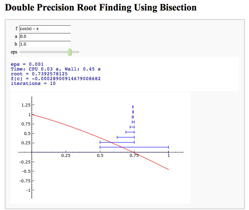
Root Finding Using Bisection
by William Stein
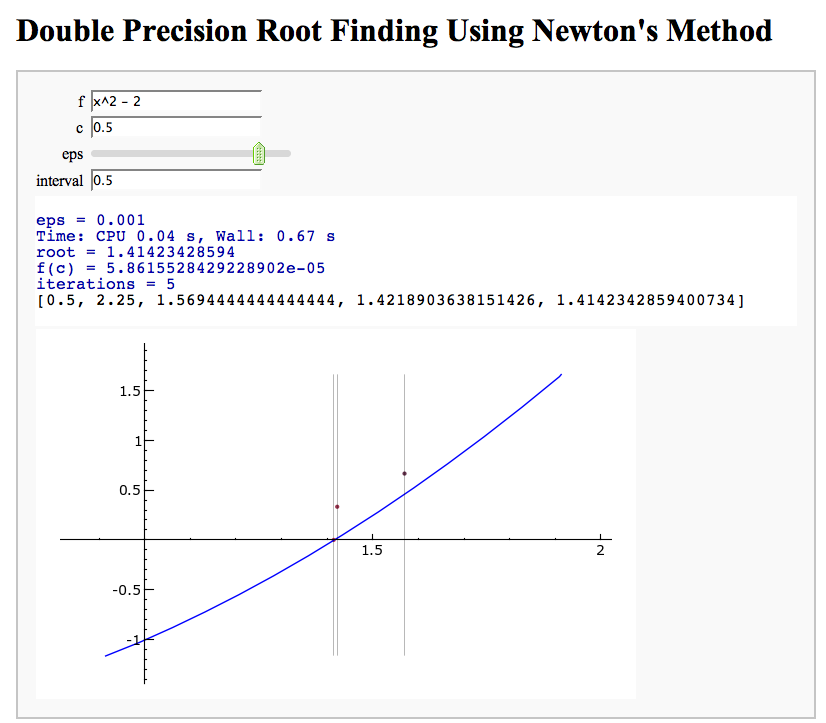
Newton's Method
Note that there is a more complicated Newton's method below.
by William Stein
http://sagenb.org/home/pub/2824/
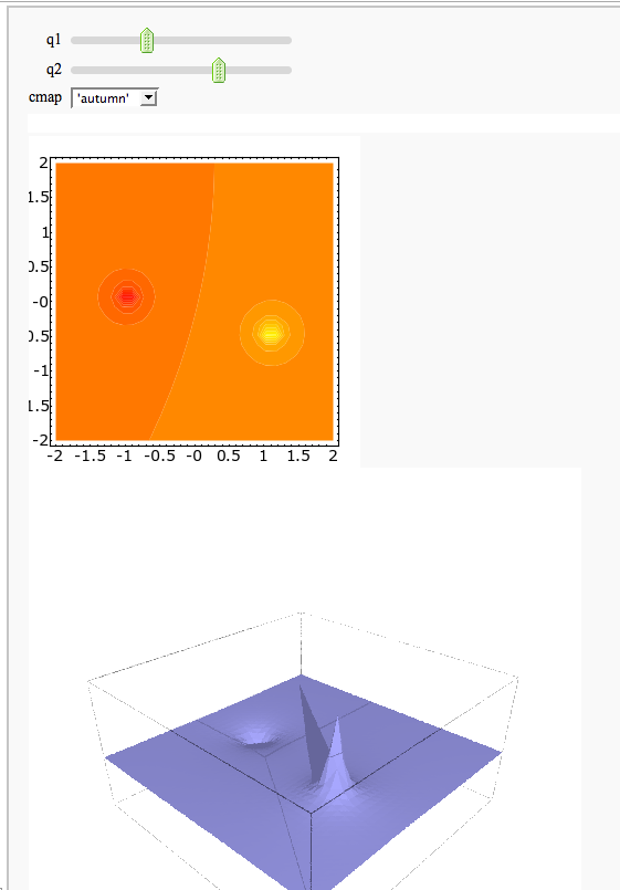
A contour map and 3d plot of two inverse distance functions
by William Stein
http://sagenb.org/home/pub/2823/
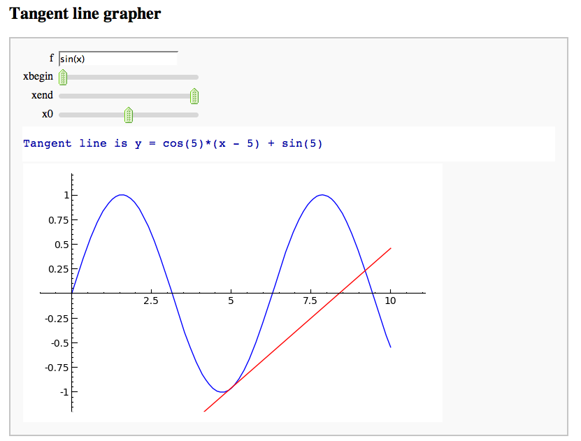
A simple tangent line grapher
by Marshall Hampton
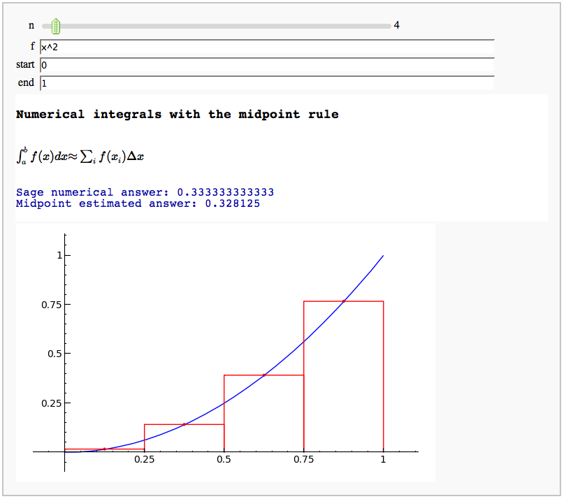
Numerical integrals with the midpoint rule
by Marshall Hampton
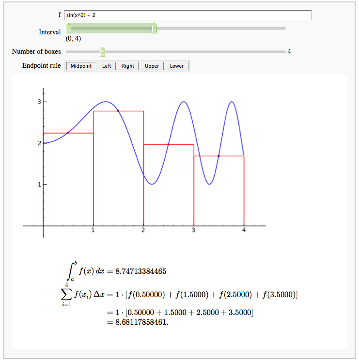
Numerical integrals with various rules
by Nick Alexander (based on the work of Marshall Hampton)
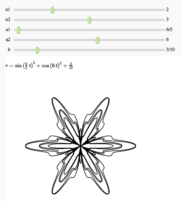
Some polar parametric curves
by Marshall Hampton. This is not very general, but could be modified to show other families of polar curves.
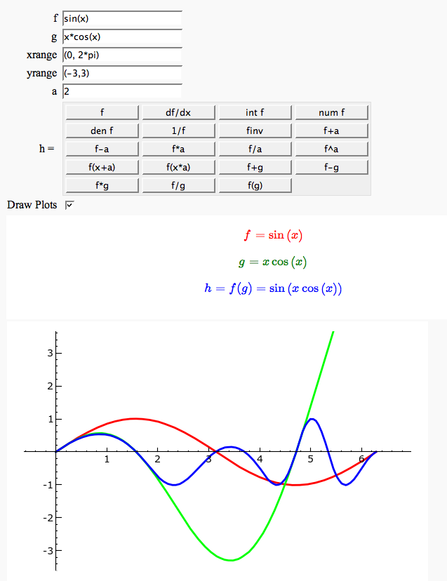
Function tool
Enter symbolic functions f, g, and a, a range, then click the appropriate button to compute and plot some combination of f, g, and a along with f and g. This is inspired by the Matlab funtool GUI.
Newton-Raphson Root Finding
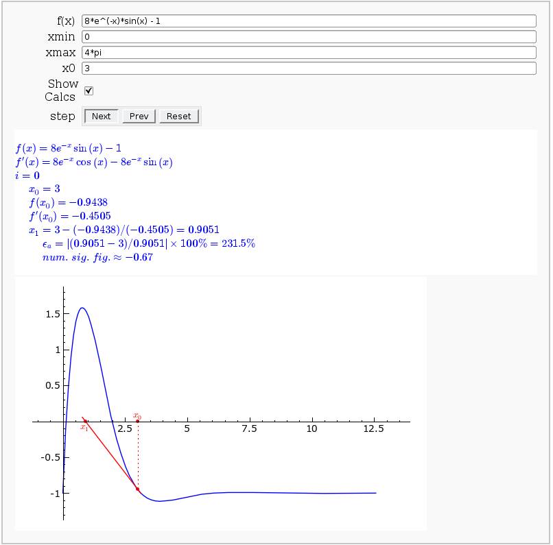
by Neal Holtz
This allows user to display the Newton-Raphson procedure one step at a time. It uses the heuristic that, if any of the values of the controls change, then the procedure should be re-started, else it should be continued.
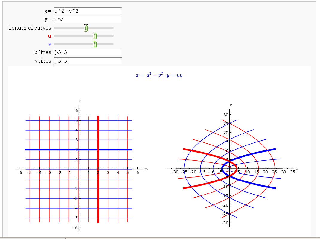
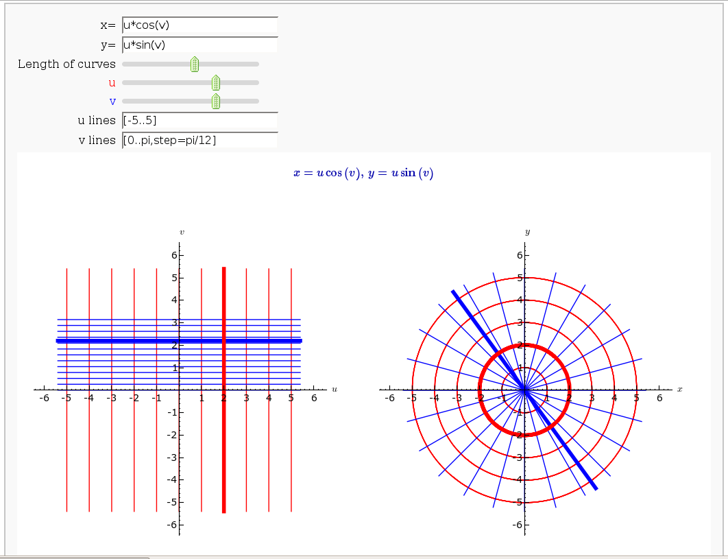
Coordinate Transformations
by Jason Grout
Taylor Series
by Harald Schilly
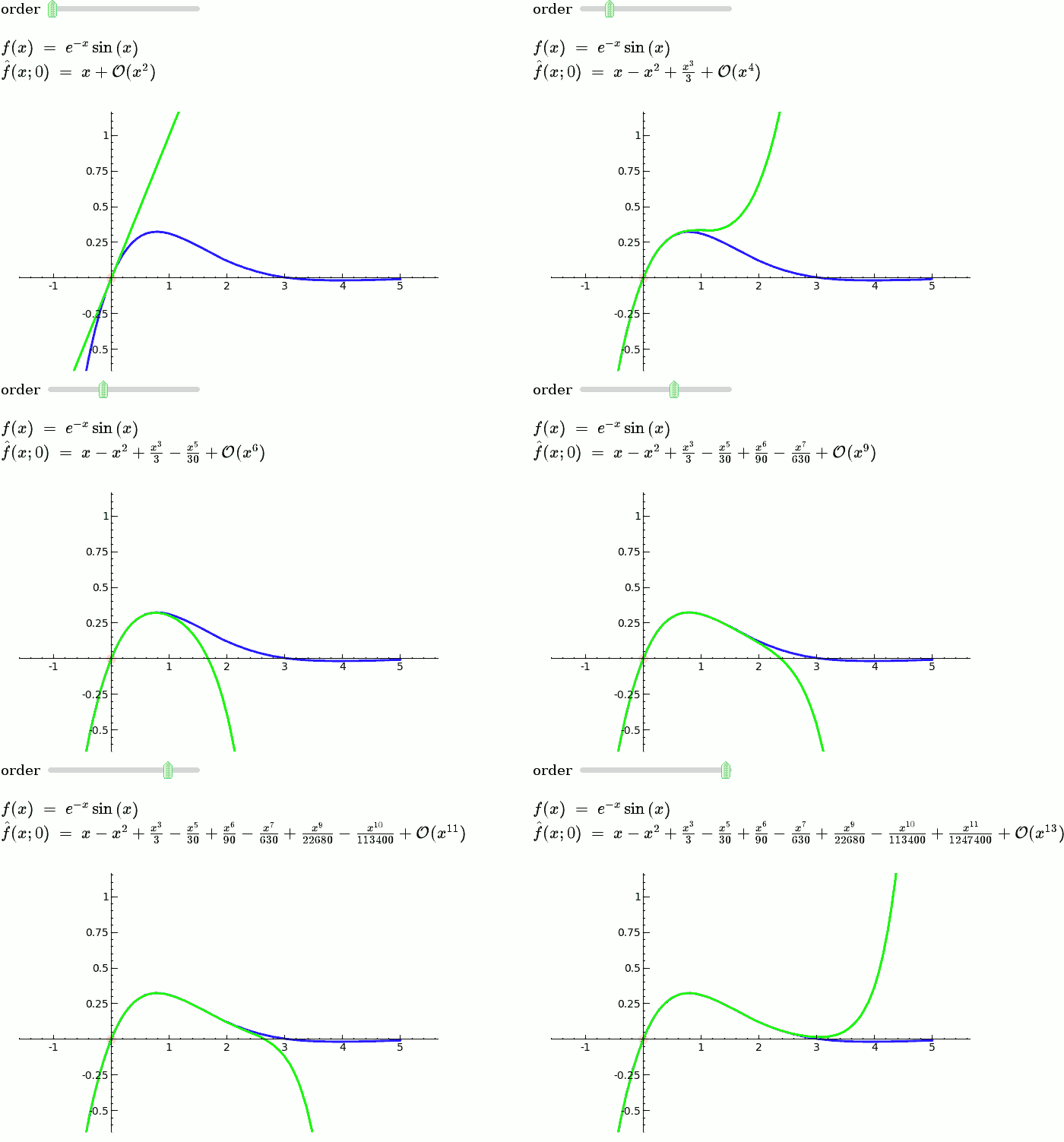
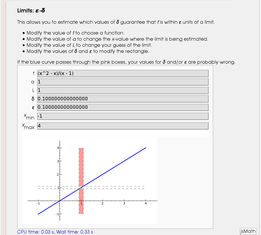
Illustration of the precise definition of a limit
by John Perry
I'll break tradition and put the image first. Apologies if this is Not A Good Thing.
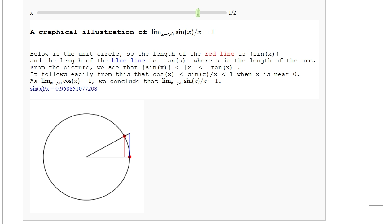
A graphical illustration of sin(x)/x -> 1 as x-> 0
by Wai Yan Pong
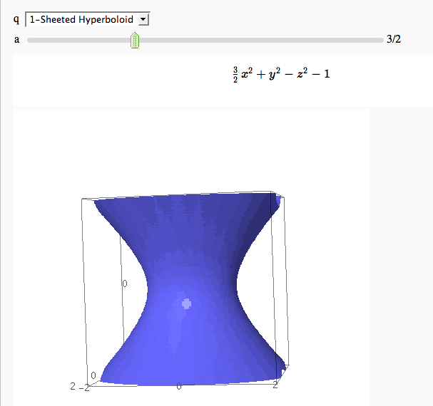
Quadric Surface Plotter
by Marshall Hampton. This is pretty simple, so I encourage people to spruce it up. In particular, it isn't set up to show all possible types of quadrics.
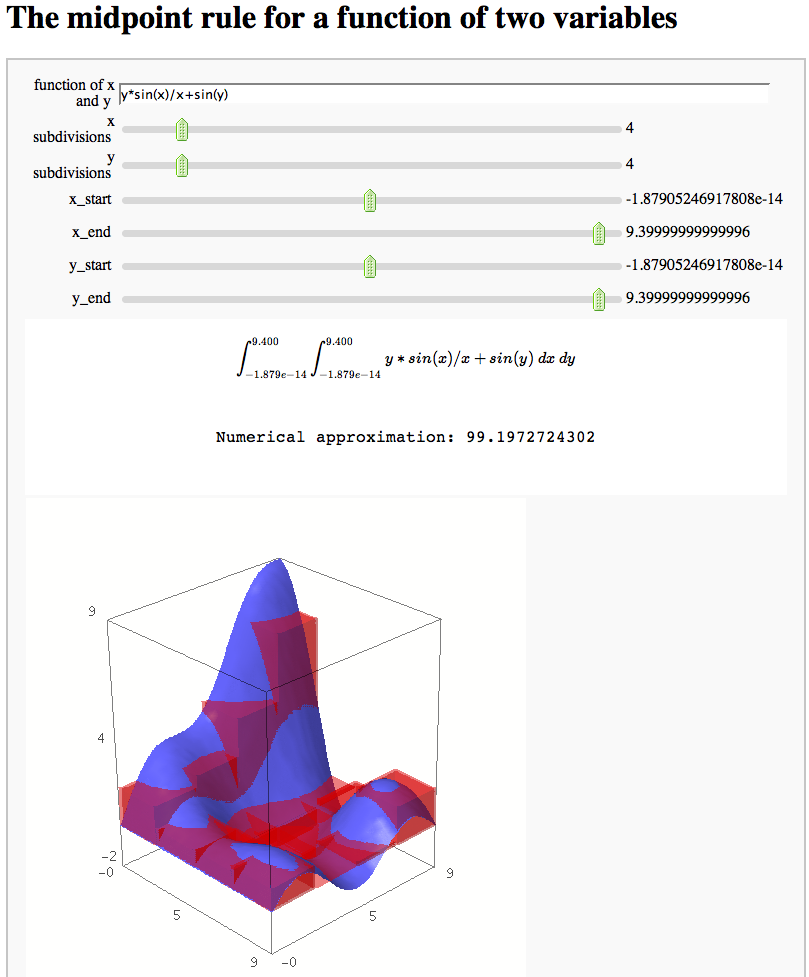
The midpoint rule for numerically integrating a function of two variables
by Marshall Hampton
Gaussian (Legendre) quadrature
by Jason Grout
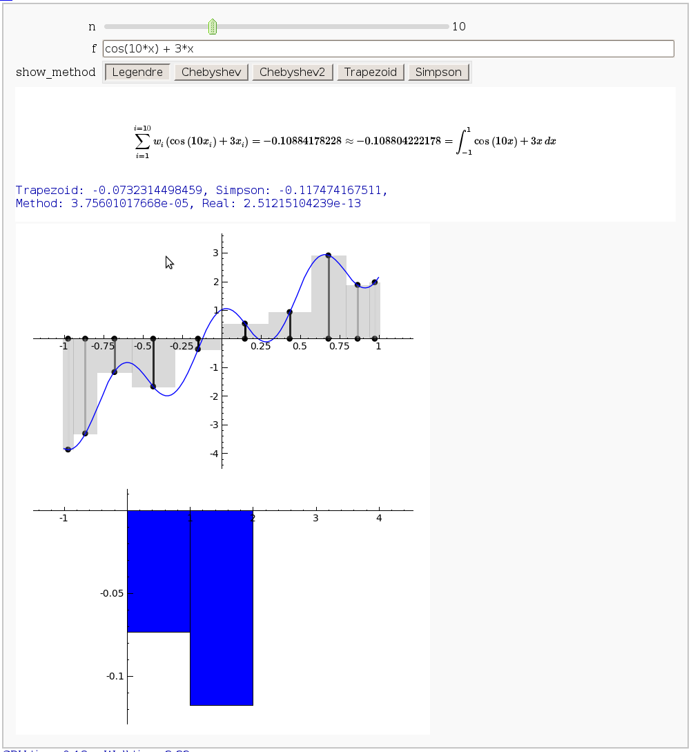
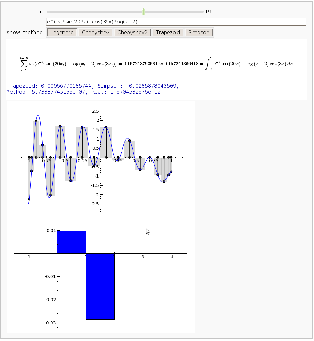
The output shows the points evaluated using Gaussian quadrature (using a weight of 1, so using Legendre polynomials). The vertical bars are shaded to represent the relative weights of the points (darker = more weight). The error in the trapezoid, Simpson, and quadrature methods is both printed out and compared through a bar graph. The "Real" error is the error returned from scipy on the definite integral.
Vector Calculus, 2-D Motion
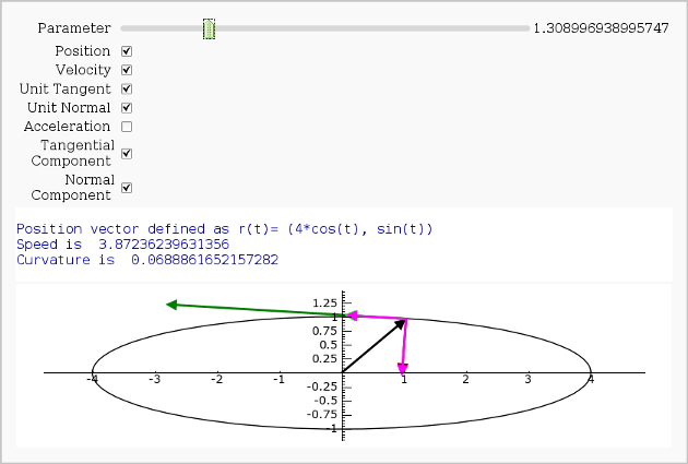
By Rob Beezer
A fast_float() version is available in a worksheet
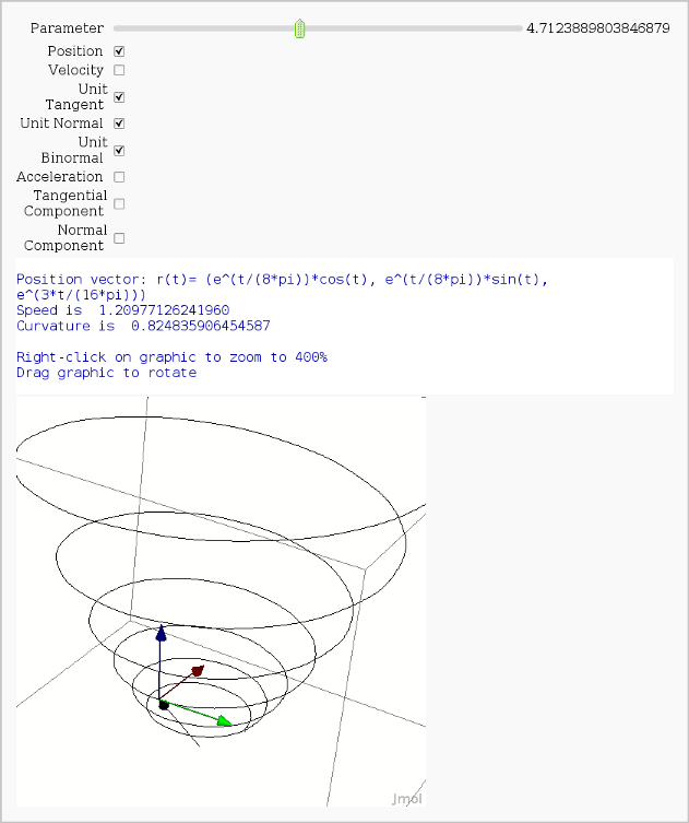
Vector Calculus, 3-D Motion
by Rob Beezer
Available as a worksheet
Multivariate Limits by Definition
by John Travis
http://www.sagenb.org/home/pub/2828/
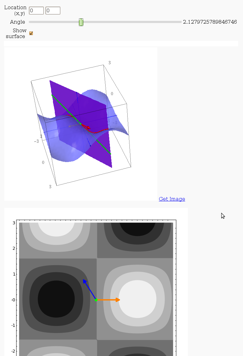
Directional Derivatives
This interact displays graphically a tangent line to a function, illustrating a directional derivative (the slope of the tangent line).
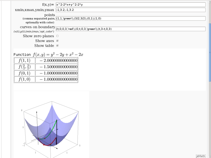
3D graph with points and curves
By Robert Marik
This sagelet is handy when showing local, constrained and absolute maxima and minima in two variables. Available as a worksheet
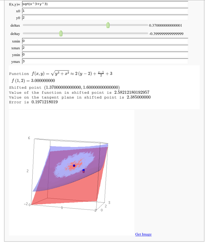
Approximating function in two variables by differential
by Robert Marik
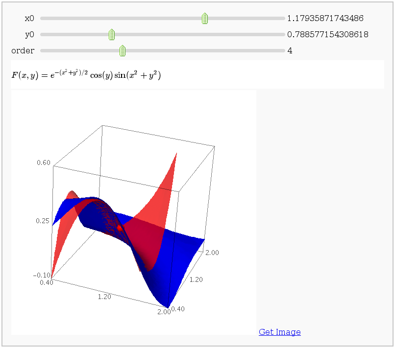
Taylor approximations in two variables
by John Palmieri
This displays the nth order Taylor approximation, for n from 1 to 10, of the function sin(x2 + y2) cos(y) exp(-(x2+y2)/2).
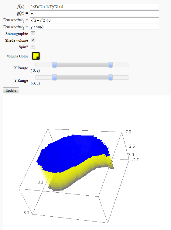
Volumes over non-rectangular domains
by John Travis
http://www.sagenb.org/home/pub/2829/
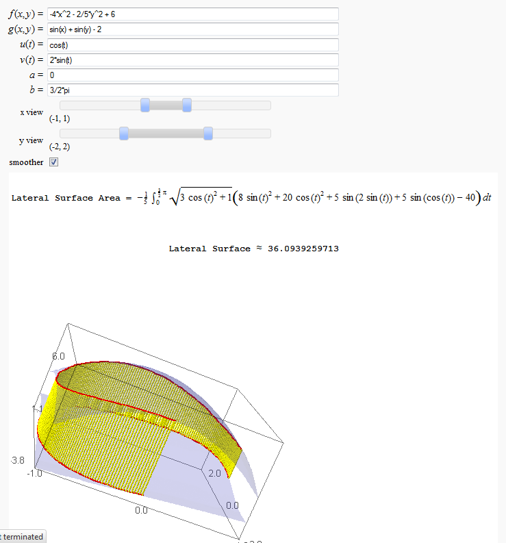
Lateral Surface Area
by John Travis
http://www.sagenb.org/home/pub/2826/
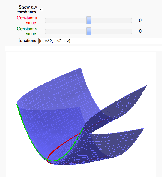
Parametric surface example
by Marshall Hampton
Line Integrals in 3D Vector Field
by John Travis
http://www.sagenb.org/home/pub/2827/
