|
Size: 57859
Comment:
|
Size: 57661
Comment: make interacts live.
|
| Deletions are marked like this. | Additions are marked like this. |
| Line 6: | Line 6: |
| {{{#!html <script type="text/javascript" src="http://aleph.sagemath.org/static/jquery.min.js"></script> <script type="text/javascript" src="http://aleph.sagemath.org/embedded_sagecell.js"></script> <script type="text/javascript">alert('hi');</script> <script> $(function() { var makecells = function() { sagecell.makeSagecell({ inputLocation: '#interact1', evalButtonText: 'Interact'}); } sagecell.init(makecells); })</script> }}} |
|
| Line 25: | Line 10: |
| {{{#!html <div id="interact1"><script type="text/code"> |
{{{#!sagecell |
| Line 65: | Line 49: |
| </script></div> | |
| Line 76: | Line 59: |
| {{{ | {{{#!sagecell |
| Line 118: | Line 101: |
| {{{ | {{{#!sagecell |
| Line 134: | Line 117: |
| {{{ | {{{#!sagecell |
| Line 154: | Line 137: |
| {{{ | {{{#!sagecell |
| Line 182: | Line 165: |
| {{{ | {{{#!sagecell |
| Line 255: | Line 238: |
| {{{ | {{{#!sagecell |
| Line 268: | Line 251: |
| {{{ | {{{#!sagecell |
| Line 366: | Line 349: |
| {{{ | {{{#!sagecell |
| Line 472: | Line 455: |
| {{{ | {{{#!sagecell |
| Line 514: | Line 497: |
| {{{ | {{{#!sagecell |
| Line 537: | Line 520: |
| {{{ | {{{#!sagecell |
| Line 564: | Line 547: |
| {{{ | {{{#!sagecell |
| Line 590: | Line 573: |
| {{{ | {{{#!sagecell |
| Line 605: | Line 588: |
| {{{ | {{{#!sagecell |
| Line 651: | Line 634: |
| {{{ from scipy.special.orthogonal import p_roots |
{{{#!sagecell import scipy import numpy from scipy.special.orthogonal import p_roots, t_roots, u_roots |
| Line 661: | Line 646: |
| 'Chebyshev': {'w': 1/sqrt(1-x**2), 'xmin': -1, 'xmax': 1, 'func': t_roots}, 'Chebyshev2': {'w': sqrt(1-x**2), 'xmin': -1, 'xmax': 1, 'func': u_roots}, 'Trapezoid': {'w': 1, 'xmin': -1, 'xmax': 1, 'func': lambda n: (linspace(-1r,1,n), numpy.array([1.0r]+[2.0r]*(n-2)+[1.0r])*1.0r/n)}, 'Simpson': {'w': 1, 'xmin': -1, 'xmax': 1, 'func': lambda n: (linspace(-1r,1,n), numpy.array([1.0r]+[4.0r,2.0r]*int((n-3.0r)/2.0r)+[4.0r,1.0r])*2.0r/(3.0r*n))}} |
'Chebyshev': {'w': 1/sqrt(1-x**2), 'xmin': -1, 'xmax': 1, 'func': t_roots}, 'Chebyshev2': {'w': sqrt(1-x**2), 'xmin': -1, 'xmax': 1, 'func': u_roots}, 'Trapezoid': {'w': 1, 'xmin': -1, 'xmax': 1, 'func': lambda n: (linspace(-1r,1,n), numpy.array([1.0r]+[2.0r]*(n-2)+[1.0r])*1.0r/n)}, 'Simpson': {'w': 1, 'xmin': -1, 'xmax': 1, 'func': lambda n: (linspace(-1r,1,n), numpy.array([1.0r]+[4.0r,2.0r]*int((n-3.0r)/2.0r)+[4.0r,1.0r])*2.0r/(3.0r*n))}} |
| Line 668: | Line 656: |
| return polygon([(center-width2,0),(center+width2,0),(center+width2,height),(center-width2,height)],**kwds) | return polygon([(center-width2,0), (center+width2,0),(center+width2,height),(center-width2,height)],**kwds) |
| Line 672: | Line 661: |
| def weights(n=slider(1,30,1,default=10),f=input_box(default=3*x+cos(10*x)),show_method=["Legendre", "Chebyshev", "Chebyshev2", "Trapezoid","Simpson"]): | def weights(n=slider(1,30,1,default=10),f=input_box(default=3*x+cos(10*x),type=SR), show_method=["Legendre", "Chebyshev", "Chebyshev2", "Trapezoid","Simpson"]): |
| Line 681: | Line 671: |
| scaled_ff = fast_float(scaled_func) | scaled_ff = fast_float(scaled_func, 'x') |
| Line 689: | Line 679: |
| stems = sum(line([(x,0),(x,scaled_ff(x))],rgbcolor=(1-y,1-y,1-y),thickness=2,markersize=6,alpha=y) for x,y in coords_scaled) points = sum([point([(x,0),(x,scaled_ff(x))],rgbcolor='black',pointsize=30) for x,_ in coords]) |
stems = sum(line([(x,0),(x,scaled_ff(x))],rgbcolor=(1-y,1-y,1-y), thickness=2,markersize=6,alpha=y) for x,y in coords_scaled) points = sum([point([(x,0), (x,scaled_ff(x))],rgbcolor='black',pointsize=30) for x,_ in coords]) |
| Line 695: | Line 687: |
| show(graph,xmin=plot_min,xmax=plot_max) | show(graph,xmin=plot_min,xmax=plot_max,aspect_ratio="auto") |
| Line 703: | Line 695: |
| html("$$\sum_{i=1}^{i=%s}w_i\left(%s\\right)= %s\\approx %s =\int_{-1}^{1}%s \,dx$$"%(n,latex(f.subs(x="x_i")), approximation, integral, latex(scaled_func))) | html("$$\sum_{i=1}^{i=%s}w_i\left(%s\\right)= %s\\approx %s =\int_{-1}^{1}%s \,dx$$"%(n, latex(f), approximation, integral, latex(scaled_func))) |
| Line 716: | Line 709: |
| {{{ | {{{#!sagecell |
| Line 828: | Line 821: |
| {{{ | {{{#!sagecell |
| Line 956: | Line 949: |
| {{{ | {{{#!sagecell |
| Line 991: | Line 984: |
| {{{ | {{{#!sagecell |
| Line 1028: | Line 1021: |
| {{{ | {{{#!sagecell |
| Line 1081: | Line 1074: |
| {{{ %hide %auto |
{{{#!sagecell |
| Line 1142: | Line 1133: |
| {{{ | {{{#!sagecell |
| Line 1180: | Line 1171: |
| {{{ | {{{#!sagecell |
| Line 1220: | Line 1211: |
| {{{ | {{{#!sagecell |
| Line 1327: | Line 1318: |
| {{{ | {{{#!sagecell |
| Line 1384: | Line 1375: |
| {{{ | {{{#!sagecell |
| Line 1405: | Line 1396: |
| {{{ | {{{#!sagecell |
Sage Interactions - Calculus
goto interact main page
Contents
-
Sage Interactions - Calculus
- Root Finding Using Bisection
- Newton's Method
- A contour map and 3d plot of two inverse distance functions
- A simple tangent line grapher
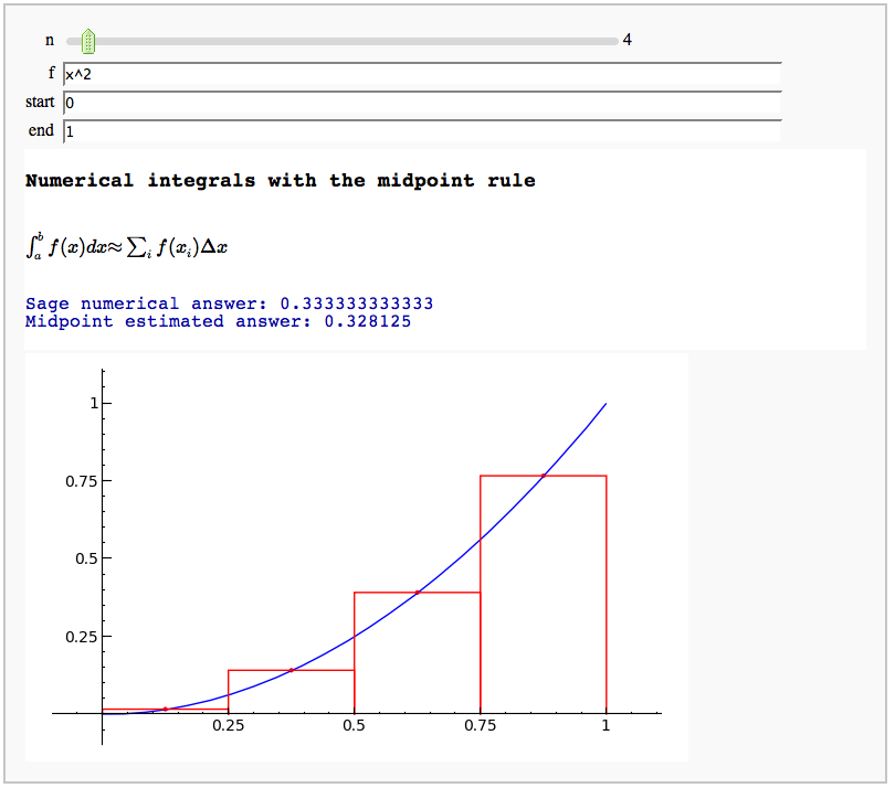
- Numerical integrals with the midpoint rule
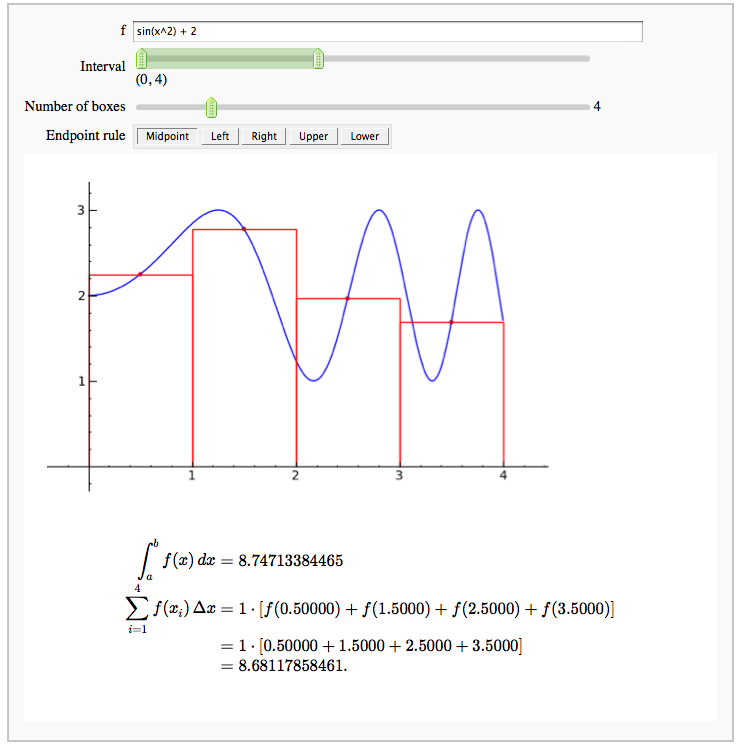
- Numerical integrals with various rules
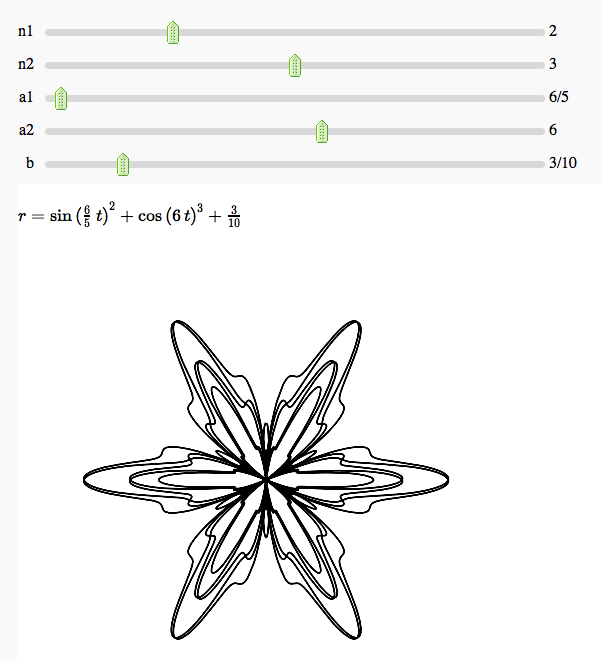
- Some polar parametric curves
- Function tool
- Newton-Raphson Root Finding
- Coordinate Transformations
- Taylor Series
- Illustration of the precise definition of a limit
- A graphical illustration of sin(x)/x -> 1 as x-> 0
- Quadric Surface Plotter
- The midpoint rule for numerically integrating a function of two variables
- Gaussian (Legendre) quadrature
- Vector Calculus, 2-D Motion
- Vector Calculus, 3-D Motion
- Multivariate Limits by Definition
- Directional Derivatives
- 3D graph with points and curves
- Approximating function in two variables by differential
- Taylor approximations in two variables
- Volumes over non-rectangular domains
- Lateral Surface Area
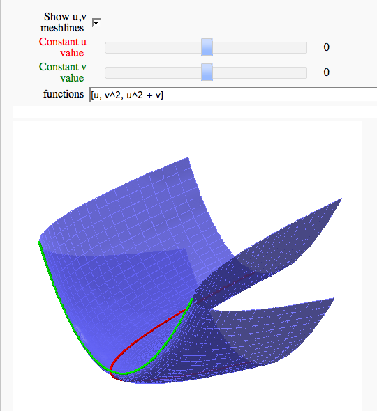
- Parametric surface example
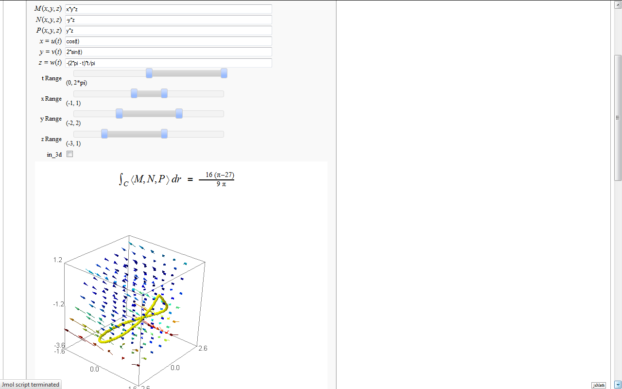
- Line Integrals in 3D Vector Field
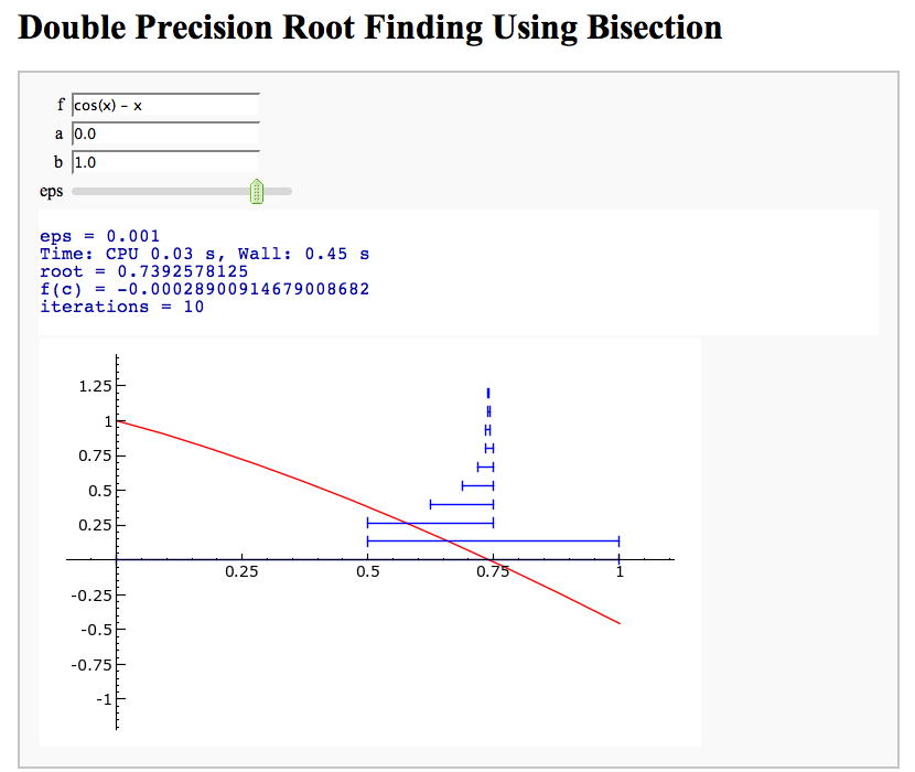
Root Finding Using Bisection
by William Stein
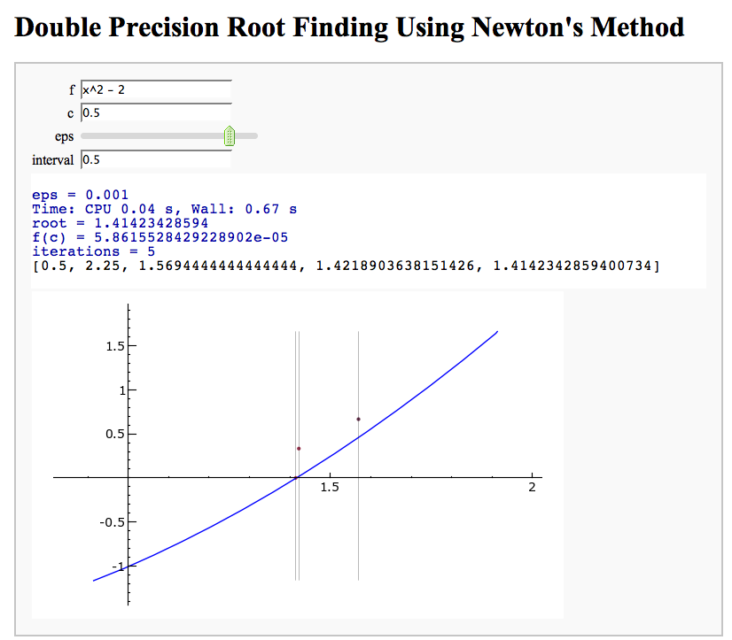
Newton's Method
Note that there is a more complicated Newton's method below.
by William Stein
http://sagenb.org/home/pub/2824/
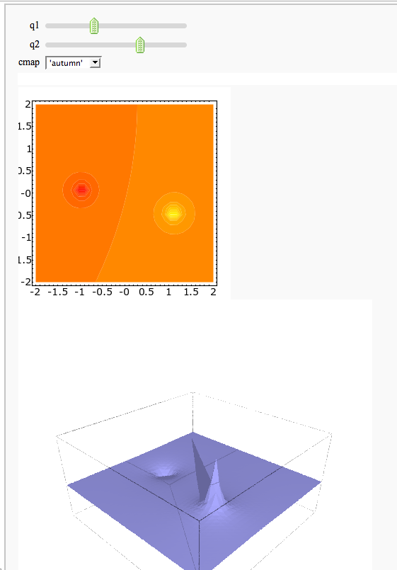
A contour map and 3d plot of two inverse distance functions
by William Stein
http://sagenb.org/home/pub/2823/
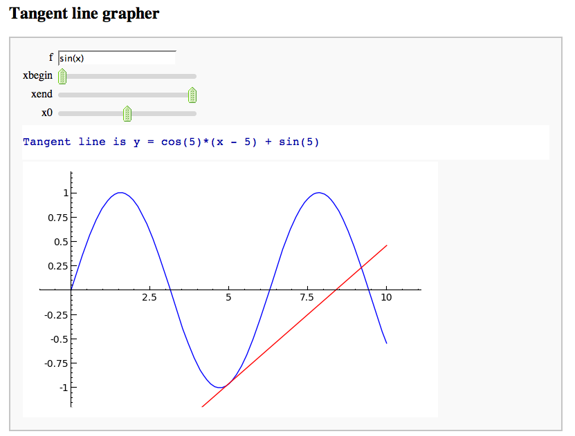
A simple tangent line grapher
by Marshall Hampton
Numerical integrals with the midpoint rule
by Marshall Hampton
Numerical integrals with various rules
by Nick Alexander (based on the work of Marshall Hampton)
Some polar parametric curves
by Marshall Hampton. This is not very general, but could be modified to show other families of polar curves.
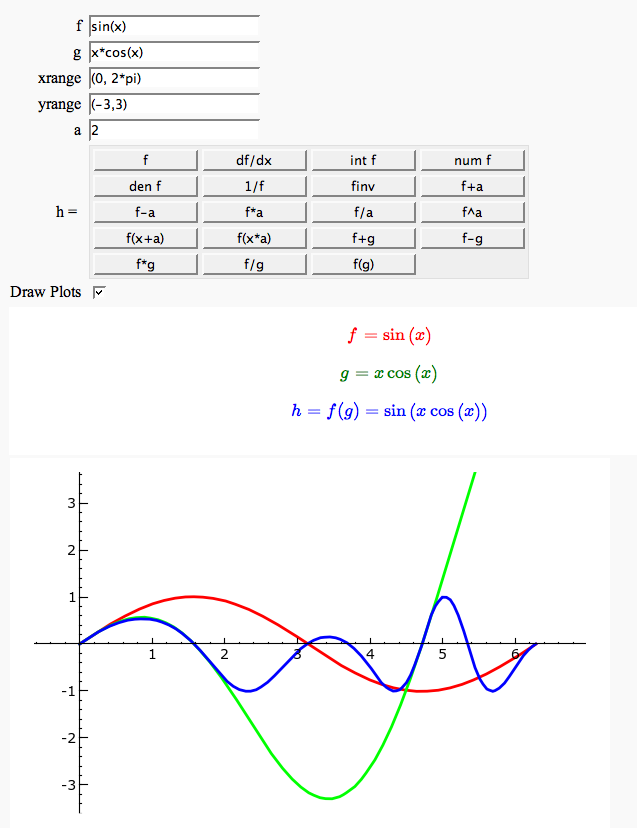
Function tool
Enter symbolic functions f, g, and a, a range, then click the appropriate button to compute and plot some combination of f, g, and a along with f and g. This is inspired by the Matlab funtool GUI.
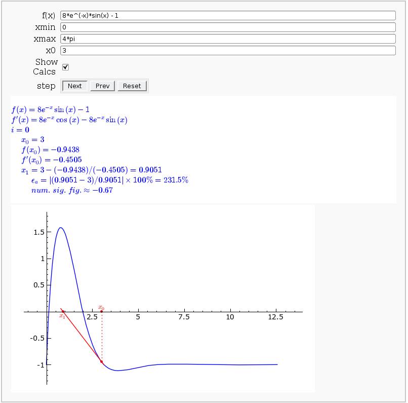
Newton-Raphson Root Finding
by Neal Holtz
This allows user to display the Newton-Raphson procedure one step at a time. It uses the heuristic that, if any of the values of the controls change, then the procedure should be re-started, else it should be continued.
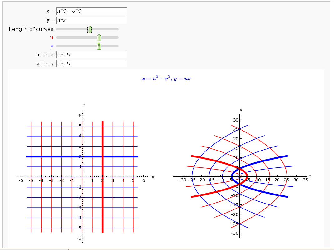
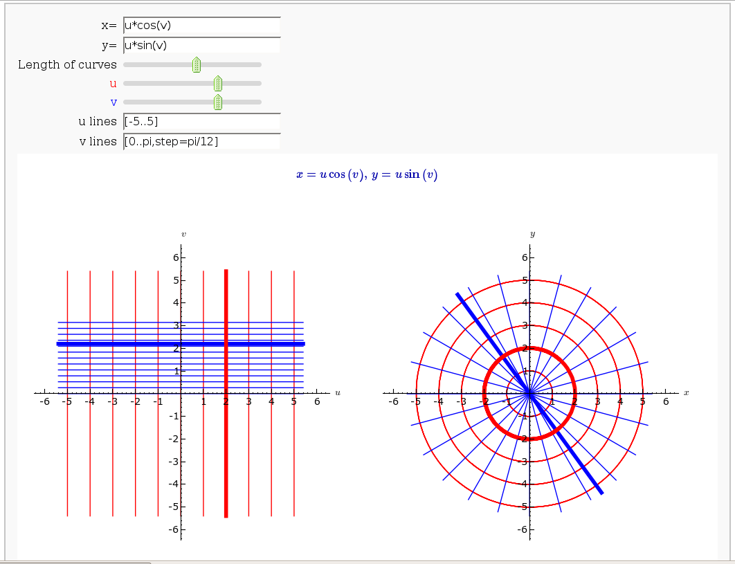
Coordinate Transformations
by Jason Grout
Taylor Series
by Harald Schilly
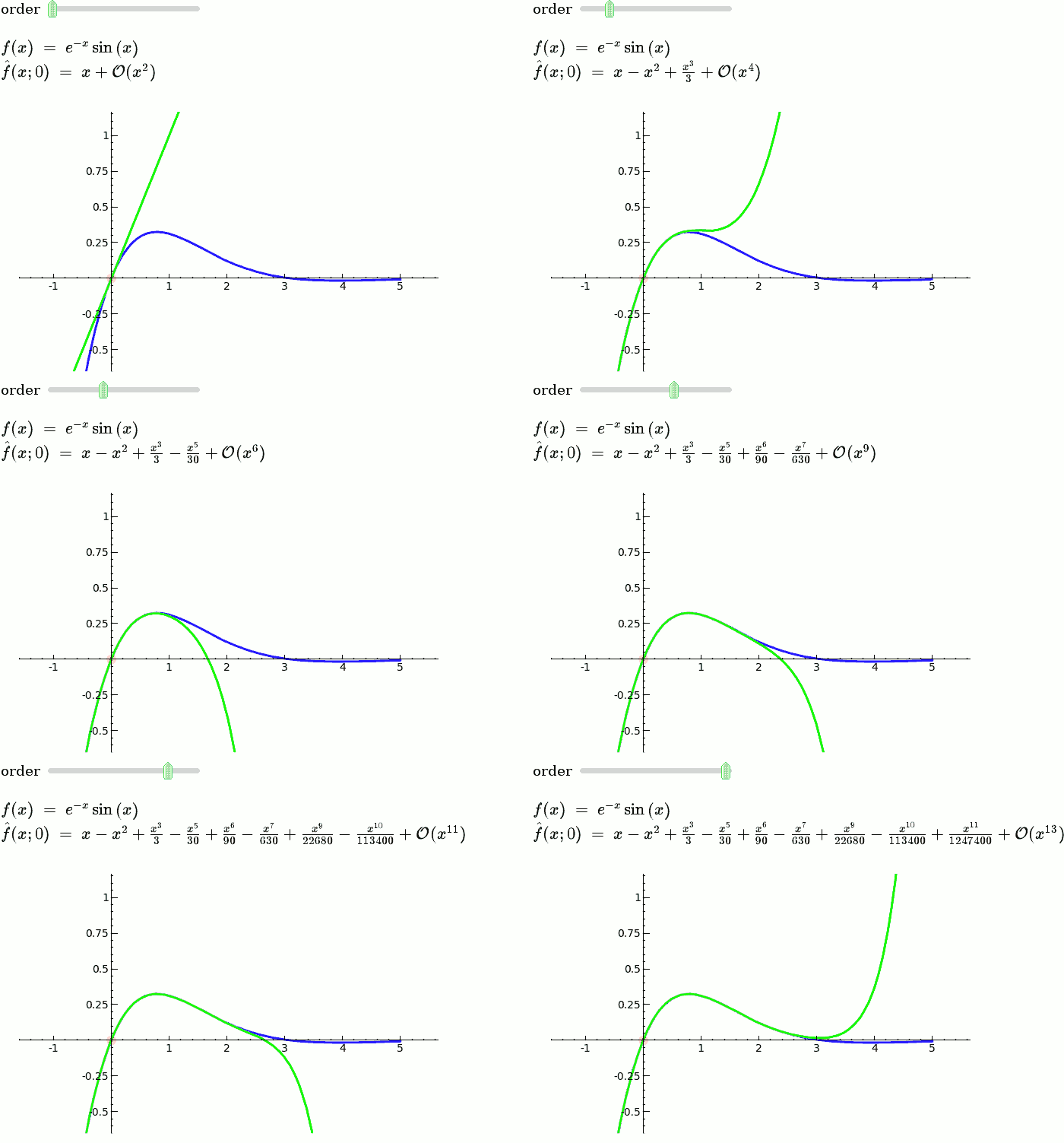
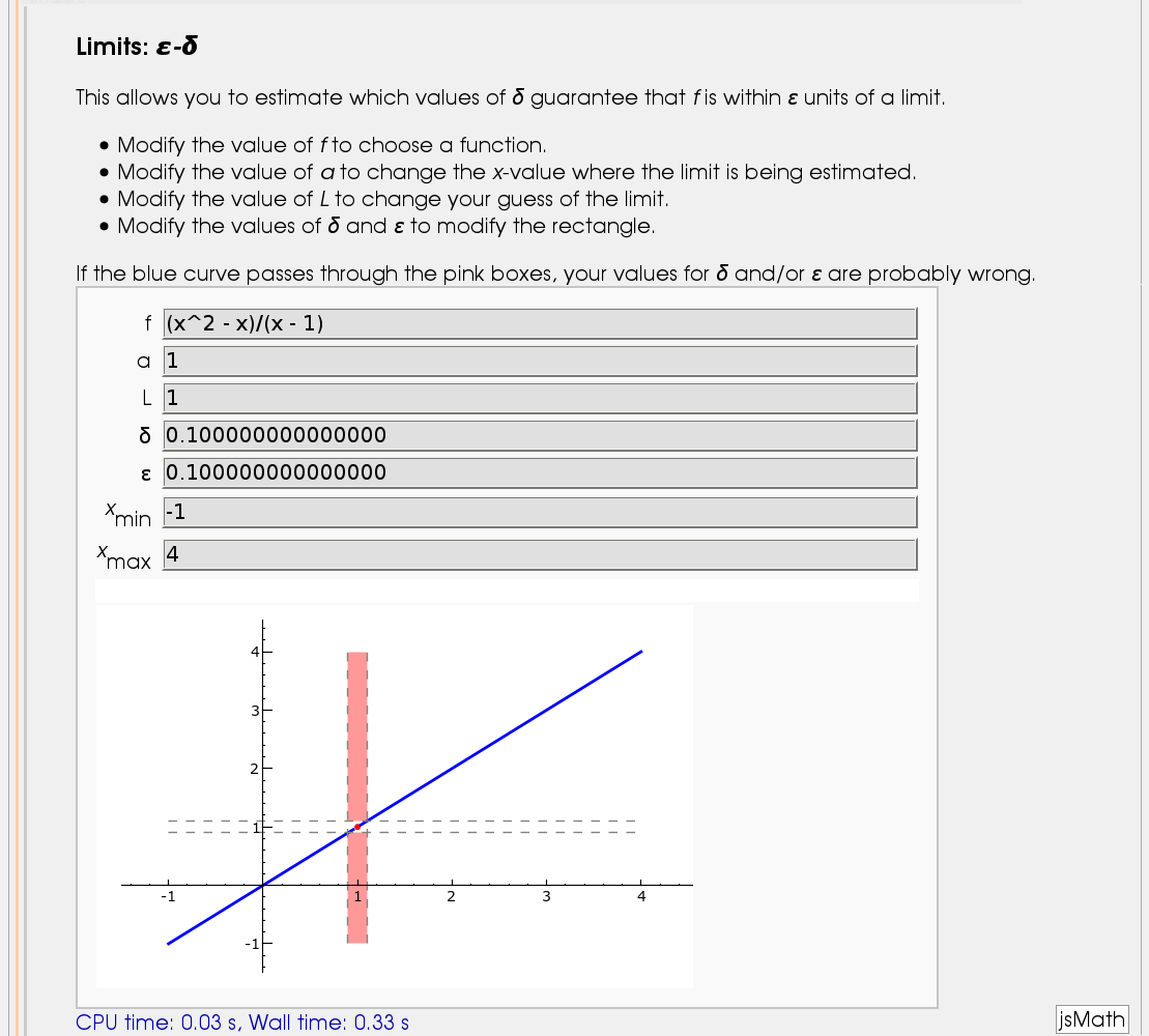
Illustration of the precise definition of a limit
by John Perry
I'll break tradition and put the image first. Apologies if this is Not A Good Thing.
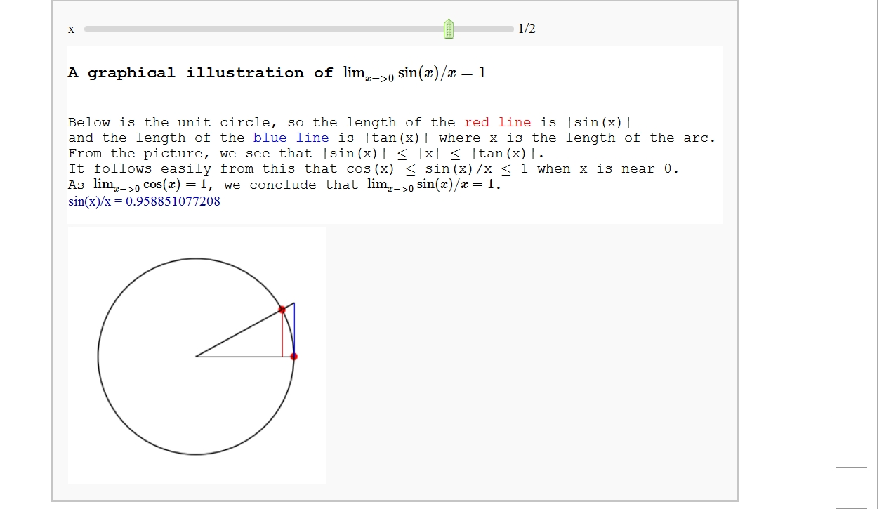
A graphical illustration of sin(x)/x -> 1 as x-> 0
by Wai Yan Pong
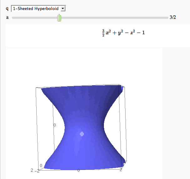
Quadric Surface Plotter
by Marshall Hampton. This is pretty simple, so I encourage people to spruce it up. In particular, it isn't set up to show all possible types of quadrics.
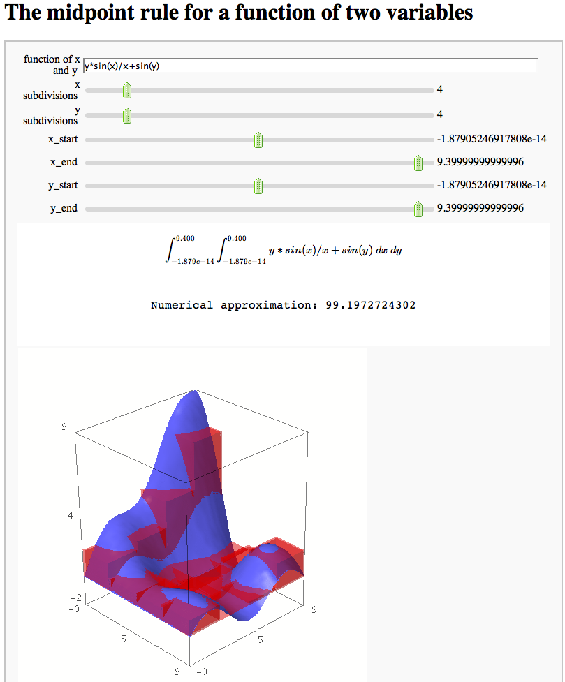
The midpoint rule for numerically integrating a function of two variables
by Marshall Hampton
Gaussian (Legendre) quadrature
by Jason Grout
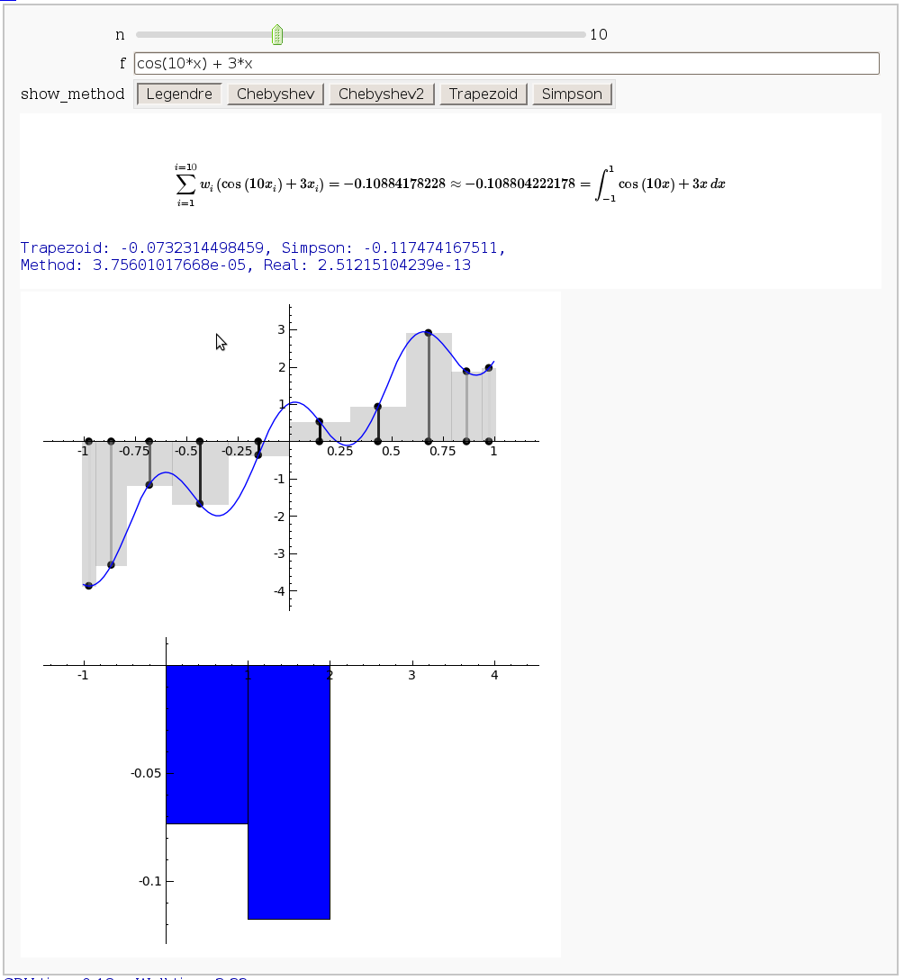
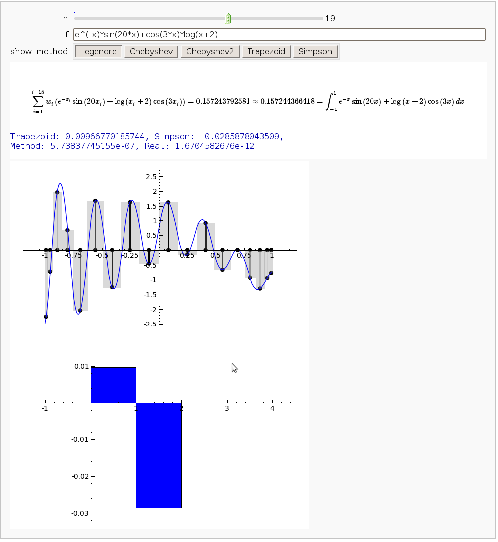
The output shows the points evaluated using Gaussian quadrature (using a weight of 1, so using Legendre polynomials). The vertical bars are shaded to represent the relative weights of the points (darker = more weight). The error in the trapezoid, Simpson, and quadrature methods is both printed out and compared through a bar graph. The "Real" error is the error returned from scipy on the definite integral.
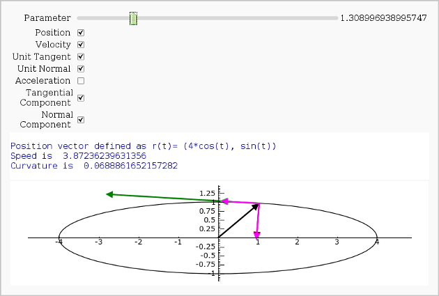
Vector Calculus, 2-D Motion
By Rob Beezer
A fast_float() version is available in a worksheet
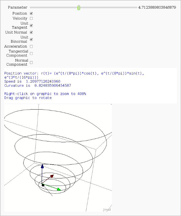
Vector Calculus, 3-D Motion
by Rob Beezer
Available as a worksheet
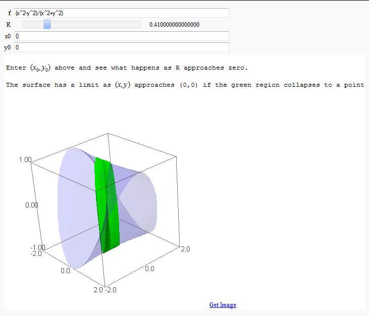
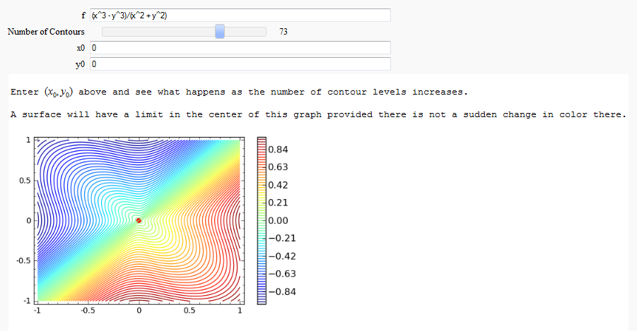
Multivariate Limits by Definition
by John Travis
http://www.sagenb.org/home/pub/2828/
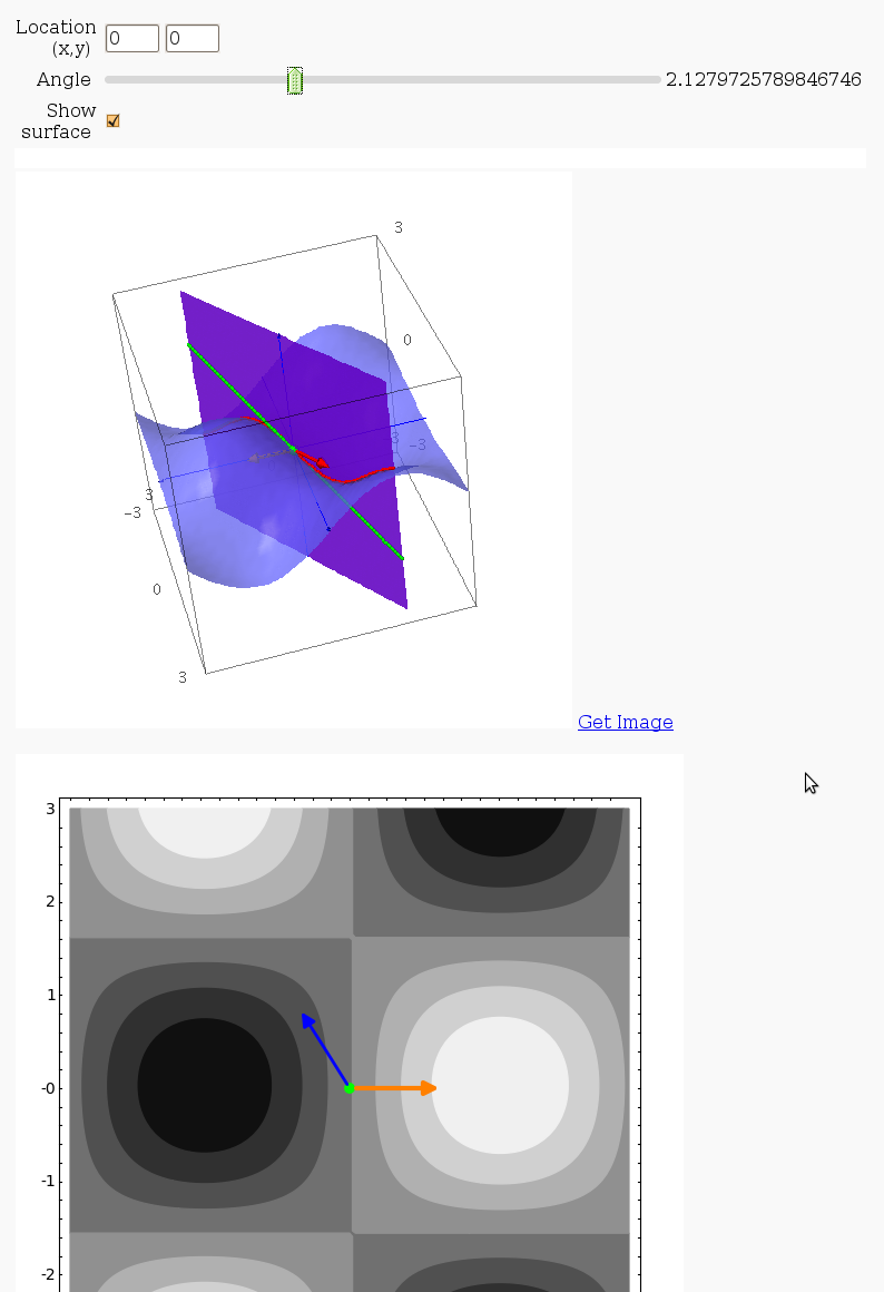
Directional Derivatives
This interact displays graphically a tangent line to a function, illustrating a directional derivative (the slope of the tangent line).
3D graph with points and curves
By Robert Marik
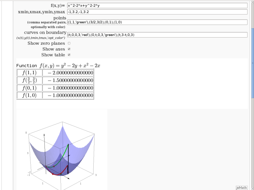
This sagelet is handy when showing local, constrained and absolute maxima and minima in two variables. Available as a worksheet
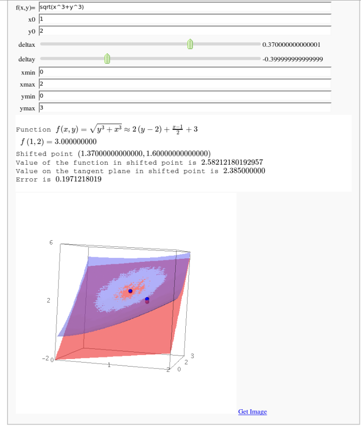
Approximating function in two variables by differential
by Robert Marik
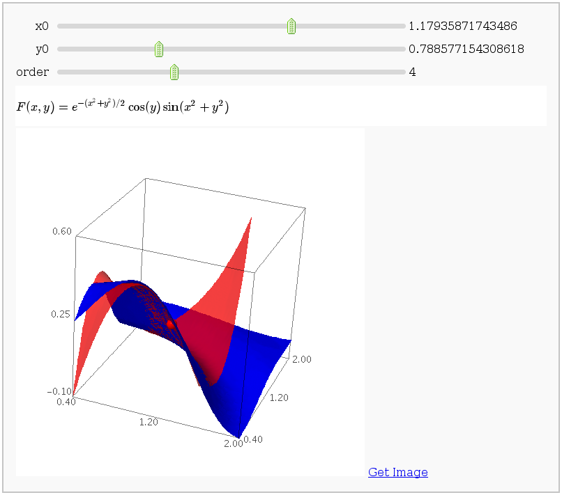
Taylor approximations in two variables
by John Palmieri
This displays the nth order Taylor approximation, for n from 1 to 10, of the function sin(x2 + y2) cos(y) exp(-(x2+y2)/2).
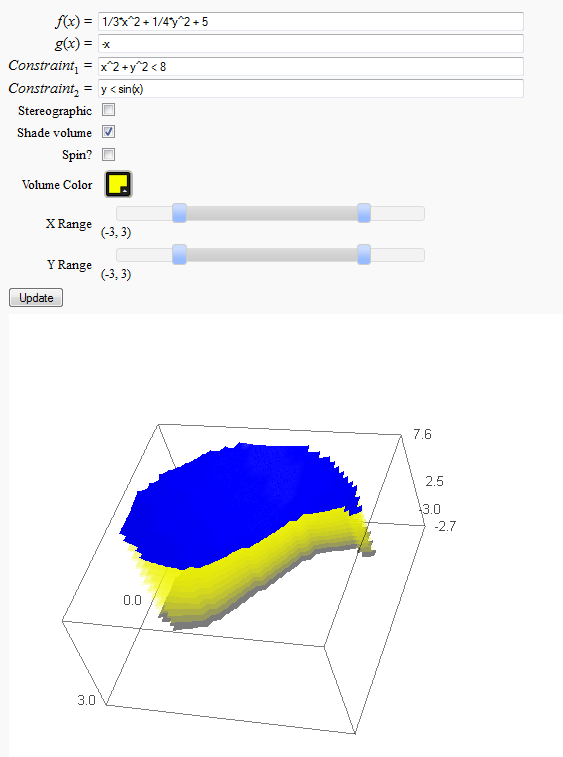
Volumes over non-rectangular domains
by John Travis
http://www.sagenb.org/home/pub/2829/
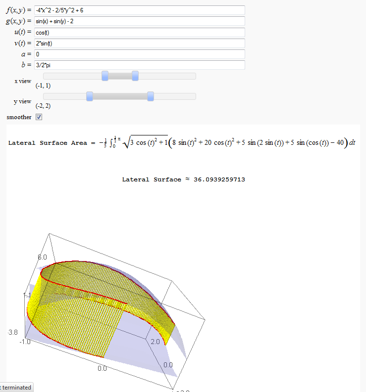
Lateral Surface Area
by John Travis
http://www.sagenb.org/home/pub/2826/
Parametric surface example
by Marshall Hampton
Line Integrals in 3D Vector Field
by John Travis
http://www.sagenb.org/home/pub/2827/
