|
Size: 58516
Comment:
|
Size: 62750
Comment:
|
| Deletions are marked like this. | Additions are marked like this. |
| Line 29: | Line 29: |
| html("<h1>Double Precision Root Finding Using Bisection</h1>") @interact def _(f = cos(x) - x, a = float(0), b = float(1), eps=(-3,(-16..-1))): |
pretty_print(html("<h1>Double Precision Root Finding Using Bisection</h1>")) @interact def _(f = cos(x) - x, a = float(0), b = float(1), eps=(-3,[-16..-1])): |
| Line 35: | Line 35: |
| time c, intervals = bisect_method(f, a, b, eps) | c, intervals = bisect_method(f, a, b, eps) |
| Line 57: | Line 57: |
| http://sagenb.org/home/pub/2824/ | https://cloud.sagemath.com/projects/19575ea0-317e-402b-be57-368d04c113db/files/pub/2801-2901/2824-Double%20Precision%20Root%20Finding%20Using%20Newton's%20Method.sagews |
| Line 77: | Line 77: |
| html("<h1>Double Precision Root Finding Using Newton's Method</h1>") | pretty_print(html("<h1>Double Precision Root Finding Using Newton's Method</h1>")) |
| Line 82: | Line 82: |
| time z, iterates = newton_method(f, c, eps) | z, iterates = newton_method(f, c, eps) |
| Line 87: | Line 87: |
| html(iterates) | pretty_print(html(iterates)) |
| Line 99: | Line 99: |
| http://sagenb.org/home/pub/2823/ | https://cloud.sagemath.com/projects/19575ea0-317e-402b-be57-368d04c113db/files/pub/2801-2901/2823.sagews |
| Line 118: | Line 118: |
| html('<h2>Tangent line grapher</h2>') | pretty_print(html('<h2>Tangent line grapher</h2>')) |
| Line 129: | Line 129: |
| fmax = f.find_maximum_on_interval(prange[0], prange[1])[0] fmin = f.find_minimum_on_interval(prange[0], prange[1])[0] |
fmax = f.find_local_maximum(prange[0], prange[1])[0] fmin = f.find_local_minimum(prange[0], prange[1])[0] |
| Line 138: | Line 138: |
| #find_maximum_on_interval and find_minimum_on_interval are deprecated #use find_local_maximum find_local_minimum instead #see http://trac.sagemath.org/2607 for details -RRubalcaba |
|
| Line 152: | Line 156: |
| min_y = find_minimum_on_interval(func,a,b)[0] max_y = find_maximum_on_interval(func,a,b)[0] html('<h3>Numerical integrals with the midpoint rule</h3>') html('$\int_{a}^{b}{f(x) dx} {\\approx} \sum_i{f(x_i) \Delta x}$') |
min_y = min(0, sage.numerical.optimize.find_local_minimum(func,a,b)[0]) max_y = max(0, sage.numerical.optimize.find_local_maximum(func,a,b)[0]) pretty_print(html('<h3>Numerical integrals with the midpoint rule</h3>')) pretty_print(html('$\int_{a}^{b}{f(x) dx} {\\approx} \sum_i{f(x_i) \Delta x}$')) |
| Line 167: | Line 171: |
| #find_maximum_on_interval and find_minimum_on_interval are deprecated #use find_local_maximum find_local_minimum instead #see http://trac.sagemath.org/2607 for details -RRubalcaba |
|
| Line 190: | Line 197: |
| x = find_maximum_on_interval(func, q*dx + a, q*dx + dx + a)[1] | x = find_local_maximum(func, q*dx + a, q*dx + dx + a)[1] |
| Line 193: | Line 200: |
| x = find_minimum_on_interval(func, q*dx + a, q*dx + dx + a)[1] | x = find_local_minimum(func, q*dx + a, q*dx + dx + a)[1] |
| Line 204: | Line 211: |
| min_y = min(0, find_minimum_on_interval(func,a,b)[0]) max_y = max(0, find_maximum_on_interval(func,a,b)[0]) |
min_y = min(0, find_local_minimum(func,a,b)[0]) max_y = max(0, find_local_maximum(func,a,b)[0]) |
| Line 221: | Line 228: |
| html(r''' | pretty_print(html(r''' |
| Line 231: | Line 238: |
| ''' % (numerical_answer, number_of_subdivisions, sum_html, num_html, estimated_answer)) | ''' % (numerical_answer, number_of_subdivisions, sum_html, num_html, estimated_answer))) |
| Line 451: | Line 458: |
| == Coordinate Transformations == | == Coordinate Transformations (FIXME in Jupyter) == |
| Line 513: | Line 520: |
| html.table([[uvplot,xyplot]])}}} | pretty_print(table([[uvplot,xyplot]])) }}} |
| Line 631: | Line 639: |
| sin,cos = math.sin,math.cos | |
| Line 764: | Line 772: |
| velocity = derivative( position(t) ) acceleration = derivative(velocity(t)) |
velocity = derivative(position(t), t) acceleration = derivative(velocity(t), t) |
| Line 767: | Line 775: |
| speed_deriv = derivative(speed) | speed_deriv = derivative(speed, t) |
| Line 769: | Line 777: |
| dT = derivative(tangent(t)) | dT = derivative(tangent(t), t) |
| Line 840: | Line 848: |
| == Vector Calculus, 3-D Motion == | == Vector Calculus, 3-D Motion (FIXME) == |
| Line 971: | Line 979: |
| http://www.sagenb.org/home/pub/2828/ | http://sagenb.mc.edu/home/pub/97/ |
| Line 981: | Line 989: |
| ## An updated version of this worksheet may be available at http://sagenb.mc.edu | |
| Line 986: | Line 993: |
| var('x,y,z') Rmin=1/10 |
|
| Line 988: | Line 996: |
| @interact def _(f=input_box(default=(x^3-y^3)/(x^2+y^2)),R=slider(0.1/10,Rmax,1/10,2),x0=(0),y0=(0)): |
@interact(layout=dict(top=[['f'],['x0'],['y0']], bottom=[['in_3d','curves','R','graphjmol']])) def _(f=input_box((x^2-y^2)/(x^2+y^2),width=30,label='$f(x)$'), R=slider(Rmin,Rmax,1/10,Rmax,label=', $R$'), x0=input_box(0,width=10,label='$x_0$'), y0=input_box(0,width=10,label='$y_0$'), curves=checkbox(default=false,label='Show curves'), in_3d=checkbox(default=false,label='3D'), graphjmol=checkbox(default=true,label='Interactive graph')): if graphjmol: view_method = 'jmol' else: view_method = 'tachyon' |
| Line 997: | Line 1016: |
| Line 999: | Line 1018: |
| limit = plot3d(g,(t,0,2*pi),(r,1/100,R),transformation=cylinder,rgbcolor=(0,1,0)) | collapsing_surface = plot3d(g,(t,0,2*pi),(r,1/100,R),transformation=cylinder,rgbcolor=(0,1,0)) |
| Line 1001: | Line 1020: |
| show(surface+limit) print html('Enter $(x_0 ,y_0 )$ above and see what happens as R approaches zero.') print html('The surface has a limit as $(x,y)$ approaches ('+str(x0)+','+str(y0)+') if the green region collapses to a point') |
G = surface+collapsing_surface html('Enter $(x_0 ,y_0 )$ above and see what happens as $ R \\rightarrow 0 $.') html('The surface has a limit as $(x,y) \\rightarrow $ ('+str(x0)+','+str(y0)+') if the green region collapses to a point.') # If checked, add a couple of curves on the surface corresponding to limit as x->x0 for y=x^(3/5), # and as y->y0 for x=y^(3/5). Should make this more robust but perhaps using # these relatively obtuse curves could eliminate problems. if curves: curve_x = parametric_plot3d([x0-t,y0-t^(3/5),f(x=x0-t,y=y0-t^(3/5))],(t,Rmin,Rmax),color='red',thickness=10) curve_y = parametric_plot3d([x0+t^(3/5),y0+t,f(x=x0+t^(3/5),y=y0+t)],(t,Rmin,Rmax),color='red',thickness=10) R2 = Rmin/4 G += arrow((x0-Rmin,y0-Rmin^(3/5),f(x=x0-Rmin,y=y0-Rmin^(3/5))),(x0-R2,y0-R2^(3/5),f(x=x0-R2,y=y0-R2^(3/5))),size=30 ) G += arrow((x0+Rmin^(3/5),y0+Rmin,f(x=x0+Rmin^(3/5),y=y0+Rmin)),(x0+R2^(3/5),y0+R2,f(x=x0+R2^(3/5),y=y0+R2)),size=30 ) limit_x = limit(f(x=x0-t,y=y0-t^(3/5)),t=0) limit_y = limit(f(x=x0+t^(3/5),y=y0+t),t=0) text_x = text3d(limit_x,(x0,y0,limit_x)) text_y = text3d(limit_y,(x0,y0,limit_y)) G += curve_x+curve_y+text_x+text_y html('The red curves represent a couple of trajectories on the surface. If they do not meet, then') html('there is also no limit. (If computer hangs up, likely the computer can not do these limits.)') html('\n<center><font color="red">$\lim_{(x,?)\\rightarrow(x_0,y_0)} f(x,y) =%s$</font>'%str(limit_x)+' and <font color="red">$\lim_{(?,y)\\rightarrow(x_0,y_0)} f(x,y) =%s$</font></center>'%str(limit_y)) if in_3d: show(G,stereo="redcyan",viewer=view_method) else: show(G,perspective_depth=true,viewer=view_method) |
| Line 1009: | Line 1055: |
| Line 1025: | Line 1072: |
| Rmax=2 @interact def _(f=input_box(default=(x^3-y^3)/(x^2+y^2)), N=slider(5,100,1,10,label='Number of Contours'), x0=(0),y0=(0)): print html('Enter $(x_0 ,y_0 )$ above and see what happens as the number of contour levels increases.') print html('A surface will have a limit in the center of this graph provided there is not a sudden change in color there.') |
var('x,y,z,u') @interact(layout=dict(top=[['f'],['x0'],['y0']], bottom=[['N'],['R']])) def _(f=input_box(default=(x*y^2)/(x^2+y^4),width=30,label='$f(x)$'), N=slider(5,100,1,10,label='Number of Contours'), R=slider(0.1,1,0.01,1,label='Radius of circular neighborhood'), x0=input_box(0,width=10,label='$x_0$'), y0=input_box(0,width=10,label='$y_0$')): html('Enter $(x_0 ,y_0 )$ above and see what happens as the number of contour levels $\\rightarrow \infty $.') html('A surface will have a limit in the center of this graph provided there is not a sudden change in color there.') # Need to make certain the min and max contour lines are not huge due to asymptotes. If so, clip and start contours at some reasonable # values so that there are a nice collection of contours to show around the desired point. |
| Line 1035: | Line 1088: |
| surface += parametric_plot([R*cos(u),R*sin(u)],[0,2*pi],color='black') # Nice to use if f=x*y^2/(x^2 + y^4) # var('u') # surface += parametric_plot([u^2,u],[u,-1,1],color='black') |
|
| Line 1036: | Line 1093: |
| show(limit_point+surface)}}} | # show(limit_point+surface) pretty_print(table([[surface],['hi']])) }}} |
| Line 1233: | Line 1292: |
| http://www.sagenb.org/home/pub/2829/ | https://cloud.sagemath.com/projects/19575ea0-317e-402b-be57-368d04c113db/files/pub/2801-2901/2829.sagews |
| Line 1336: | Line 1395: |
| == Lateral Surface Area == | == Lateral Surface Area (FIXME in Jupyter) == |
| Line 1340: | Line 1399: |
| http://www.sagenb.org/home/pub/2826/ | http://sagenb.mc.edu/home/pub/89/ |
| Line 1347: | Line 1406: |
| ## | |
| Line 1349: | Line 1409: |
| @interact def _(f=input_box(default=6-4*x^2-y^2*2/5,label='$f(x,y) = $'), g=input_box(default=-2+sin(x)+sin(y),label='$g(x,y) = $'), u=input_box(default=cos(t),label='$u(t) = $'), v=input_box(default=2*sin(t),label='$v(t) = $'), a=input_box(default=0,label='$a = $'), b=input_box(default=3*pi/2,label='$b = $'), |
@interact(layout=dict(top=[['f','u'],['g','v']], left=[['a'],['b'],['in_3d'],['smoother']], bottom=[['xx','yy']])) def _(f=input_box(default=6-4*x^2-y^2*2/5,label='Top = $f(x,y) = $',width=30), g=input_box(default=-2+sin(x)+sin(y),label='Bottom = $g(x,y) = $',width=30), u=input_box(default=cos(t),label=' $ x = u(t) = $',width=20), v=input_box(default=2*sin(t),label=' $ y = v(t) = $',width=20), a=input_box(default=0,label='$a = $',width=10), b=input_box(default=3*pi/2,label='$b = $',width=10), |
| Line 1358: | Line 1420: |
| smoother=checkbox(default=false)): | in_3d = checkbox(default=true,label='3D'), smoother=checkbox(default=false), auto_update=true): |
| Line 1360: | Line 1424: |
| ds = sqrt(derivative(u(t),t)^2+derivative(v(t),t)^2) | ds = sqrt(derivative(u,t)^2+derivative(v,t)^2) |
| Line 1364: | Line 1428: |
| A = (f(x=u(t),y=v(t))-g(x=u(t),y=v(t)))*ds.simplify_trig().simplify() | A = (f(x=u,y=v)-g(x=u,y=v))*ds.simplify_trig().simplify() |
| Line 1369: | Line 1433: |
| line_integral = integral(A,t,a,b) | # If you want Sage to try, uncomment the lines below. # line_integral = integrate(A,t,a,b) # html(r'<align=center size=+1>Lateral Surface Area = $ %s $ </font>'%latex(line_integral)) |
| Line 1371: | Line 1439: |
| html(r'<h4 align=center>Lateral Surface Area = $ %s $ </h4>'%latex(line_integral)) html(r'<h4 align=center>Lateral Surface $ \approx $ %s</h2>'%str(line_integral_approx)) |
html(r'<font align=center size=+1>Lateral Surface $ \approx $ %s</font>'%str(line_integral_approx)) |
| Line 1381: | Line 1447: |
| G += parametric_plot3d([u,v,g(x=u(t),y=v(t))],(t,a,b),thickness=2,color='red') G += parametric_plot3d([u,v,f(x=u(t),y=v(t))],(t,a,b),thickness=2,color='red') |
G += parametric_plot3d([u,v,g(x=u,y=v)],(t,a,b),thickness=2,color='red') G += parametric_plot3d([u,v,f(x=u,y=v)],(t,a,b),thickness=2,color='red') |
| Line 1391: | Line 1457: |
| G += parametric_plot3d([u(w),v(w),s*f(x=u(w),y=v(w))+(1-s)*g(x=u(w),y=v(w))],(s,0,1),thickness=lat_thick,color='yellow',opacity=0.9) show(G,spin=true) |
G += parametric_plot3d([u(t=w),v(t=w),s*f(x=u(t=w),y=v(t=w))+(1-s)*g(x=u(t=w),y=v(t=w))],(s,0,1),thickness=lat_thick,color='yellow',opacity=0.9) if in_3d: show(G,stereo='redcyan',spin=true) else: show(G,perspective_depth=true,spin=true) |
| Line 1397: | Line 1467: |
| == Parametric surface example == | == Parametric surface example (FIXME in Jupyter) == |
| Line 1418: | Line 1488: |
| http://www.sagenb.org/home/pub/2827/ | https://cloud.sagemath.com/projects/19575ea0-317e-402b-be57-368d04c113db/files/pub/2801-2901/2827-$%20%5Cint_%7BC%7D%20%5Cleft%20%5Clangle%20M,N,P%20%5Cright%20%5Crangle%20dr%20$%20=%20$%20%25s%20$.sagews |
Sage Interactions - Calculus
goto interact main page
Contents
-
Sage Interactions - Calculus
- Root Finding Using Bisection
- Newton's Method
- A contour map and 3d plot of two inverse distance functions
- A simple tangent line grapher
- Numerical integrals with the midpoint rule
- Numerical integrals with various rules
- Some polar parametric curves
- Function tool
- Newton-Raphson Root Finding
- Coordinate Transformations (FIXME in Jupyter)
- Taylor Series
- Illustration of the precise definition of a limit
- A graphical illustration of sin(x)/x -> 1 as x-> 0
- Quadric Surface Plotter
- The midpoint rule for numerically integrating a function of two variables
- Gaussian (Legendre) quadrature
- Vector Calculus, 2-D Motion
- Vector Calculus, 3-D Motion (FIXME)
- Multivariate Limits by Definition
- Directional Derivatives
- 3D graph with points and curves
- Approximating function in two variables by differential
- Taylor approximations in two variables
- Volumes over non-rectangular domains
- Lateral Surface Area (FIXME in Jupyter)
- Parametric surface example (FIXME in Jupyter)
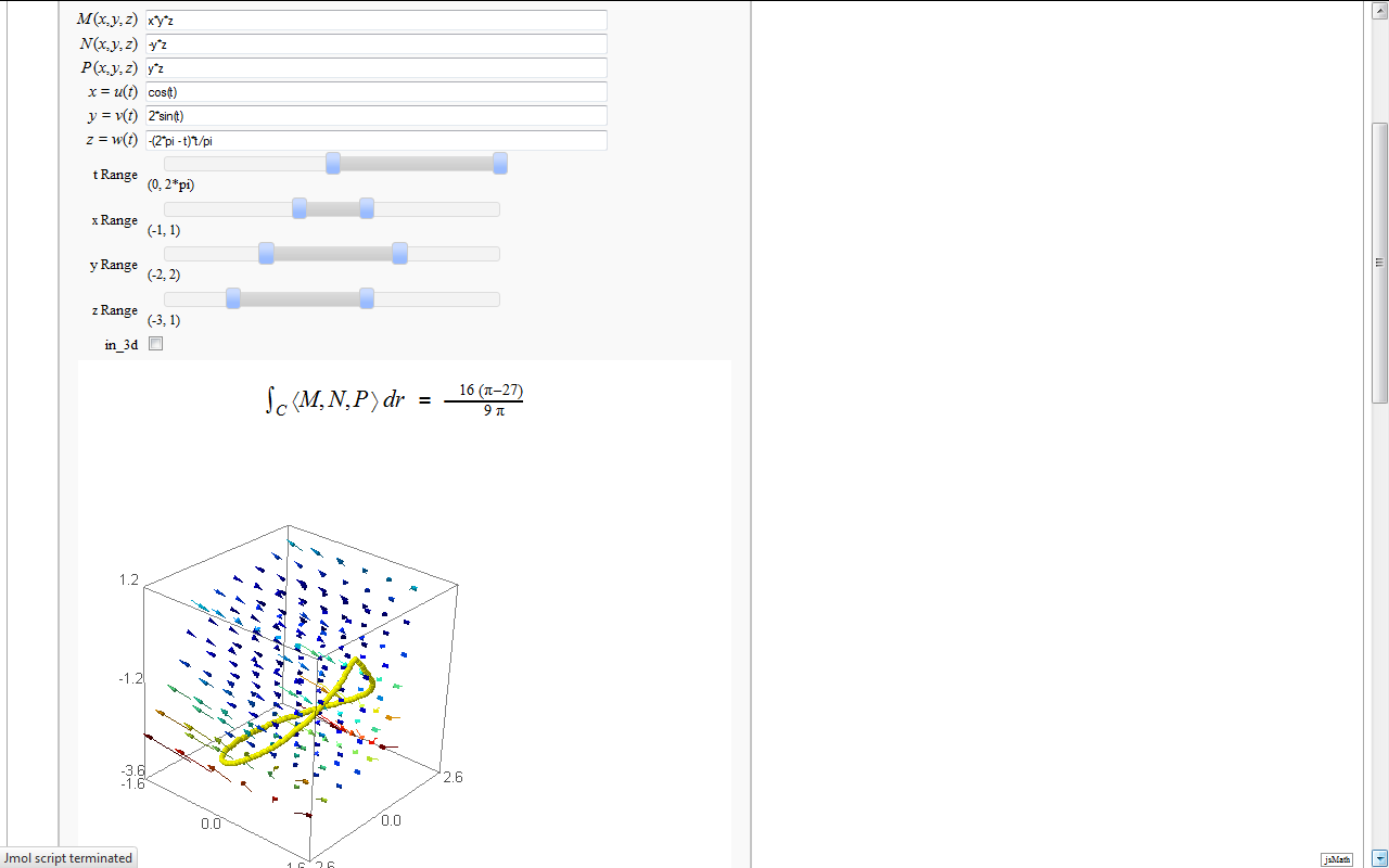
- Line Integrals in 3D Vector Field
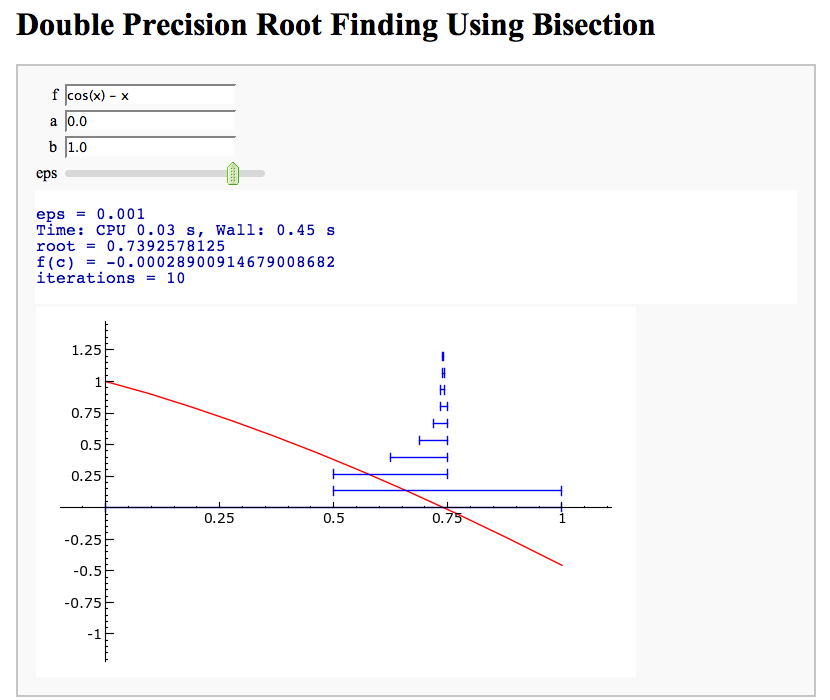
Root Finding Using Bisection
by William Stein
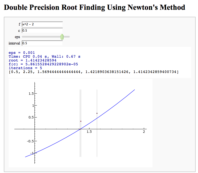
Newton's Method
Note that there is a more complicated Newton's method below.
by William Stein
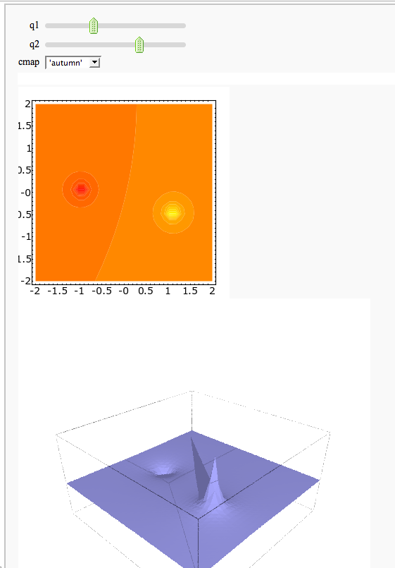
A contour map and 3d plot of two inverse distance functions
by William Stein
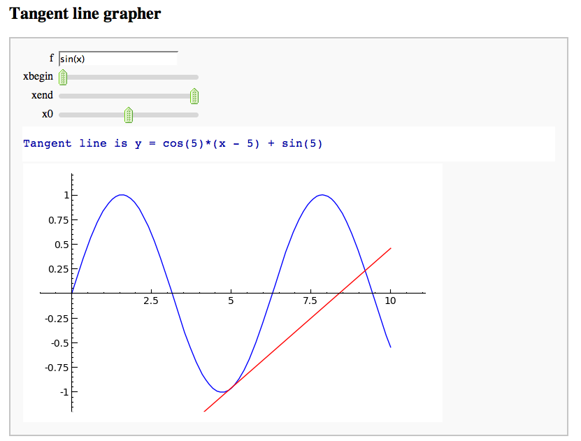
A simple tangent line grapher
by Marshall Hampton
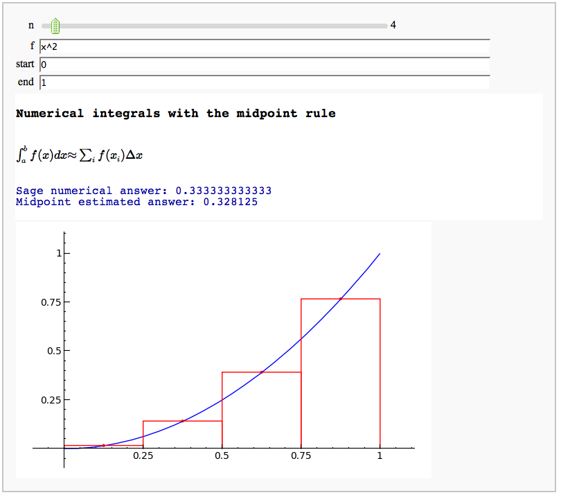
Numerical integrals with the midpoint rule
by Marshall Hampton
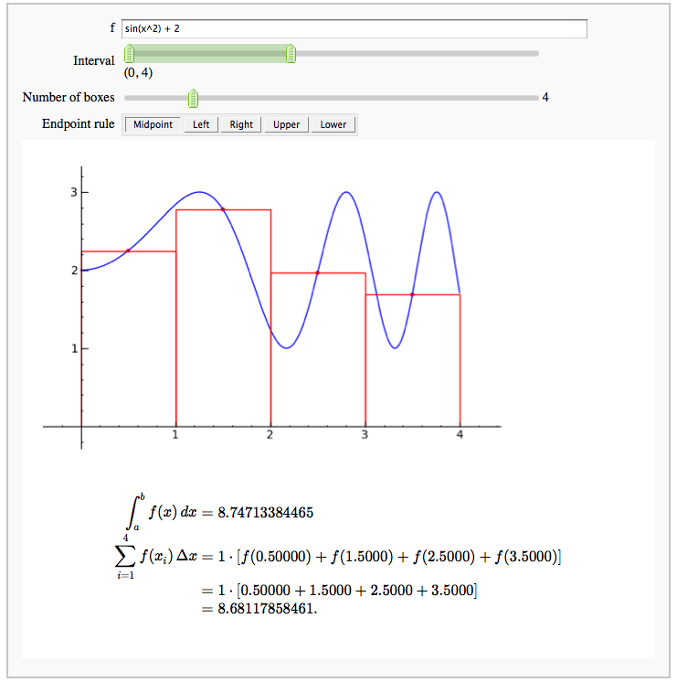
Numerical integrals with various rules
by Nick Alexander (based on the work of Marshall Hampton)
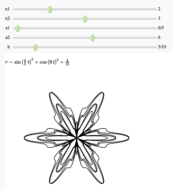
Some polar parametric curves
by Marshall Hampton. This is not very general, but could be modified to show other families of polar curves.
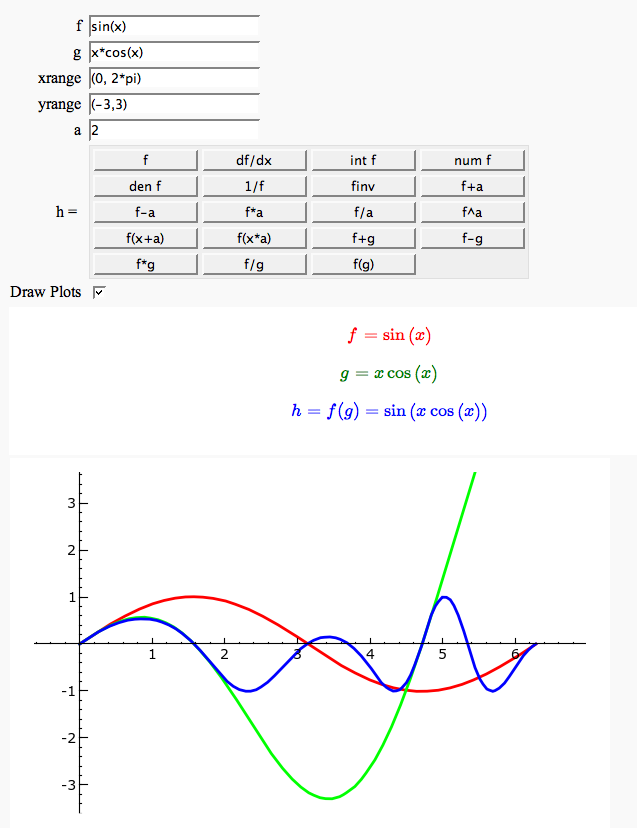
Function tool
Enter symbolic functions f, g, and a, a range, then click the appropriate button to compute and plot some combination of f, g, and a along with f and g. This is inspired by the Matlab funtool GUI.
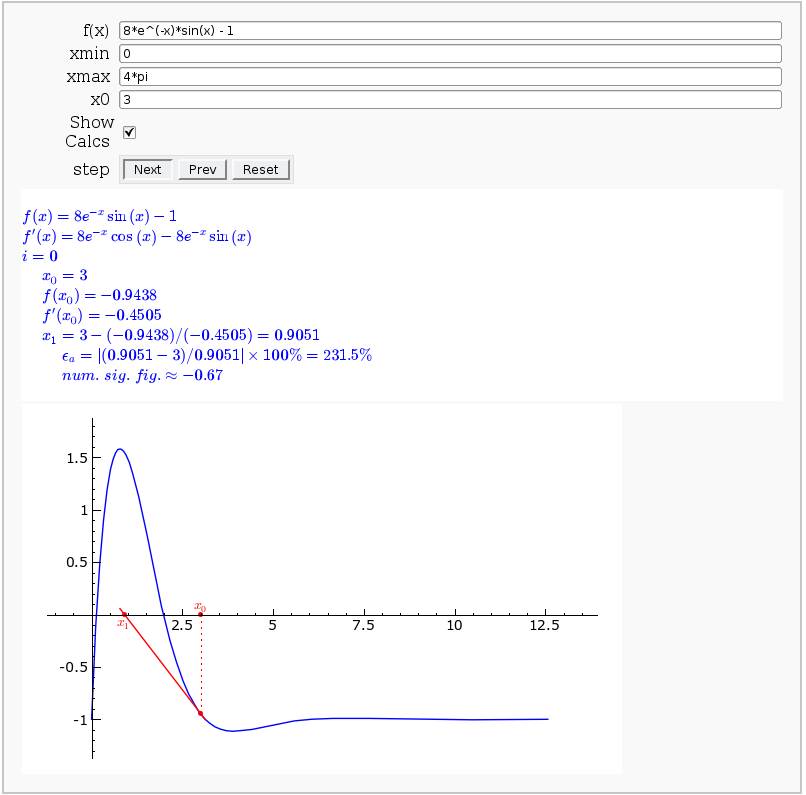
Newton-Raphson Root Finding
by Neal Holtz
This allows user to display the Newton-Raphson procedure one step at a time. It uses the heuristic that, if any of the values of the controls change, then the procedure should be re-started, else it should be continued.
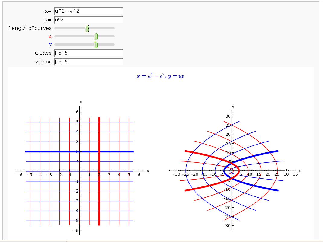
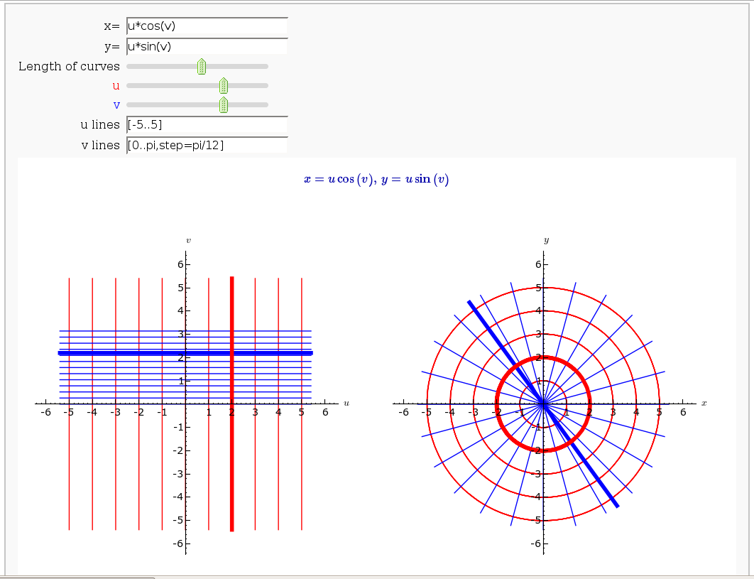
Coordinate Transformations (FIXME in Jupyter)
by Jason Grout
Taylor Series
by Harald Schilly
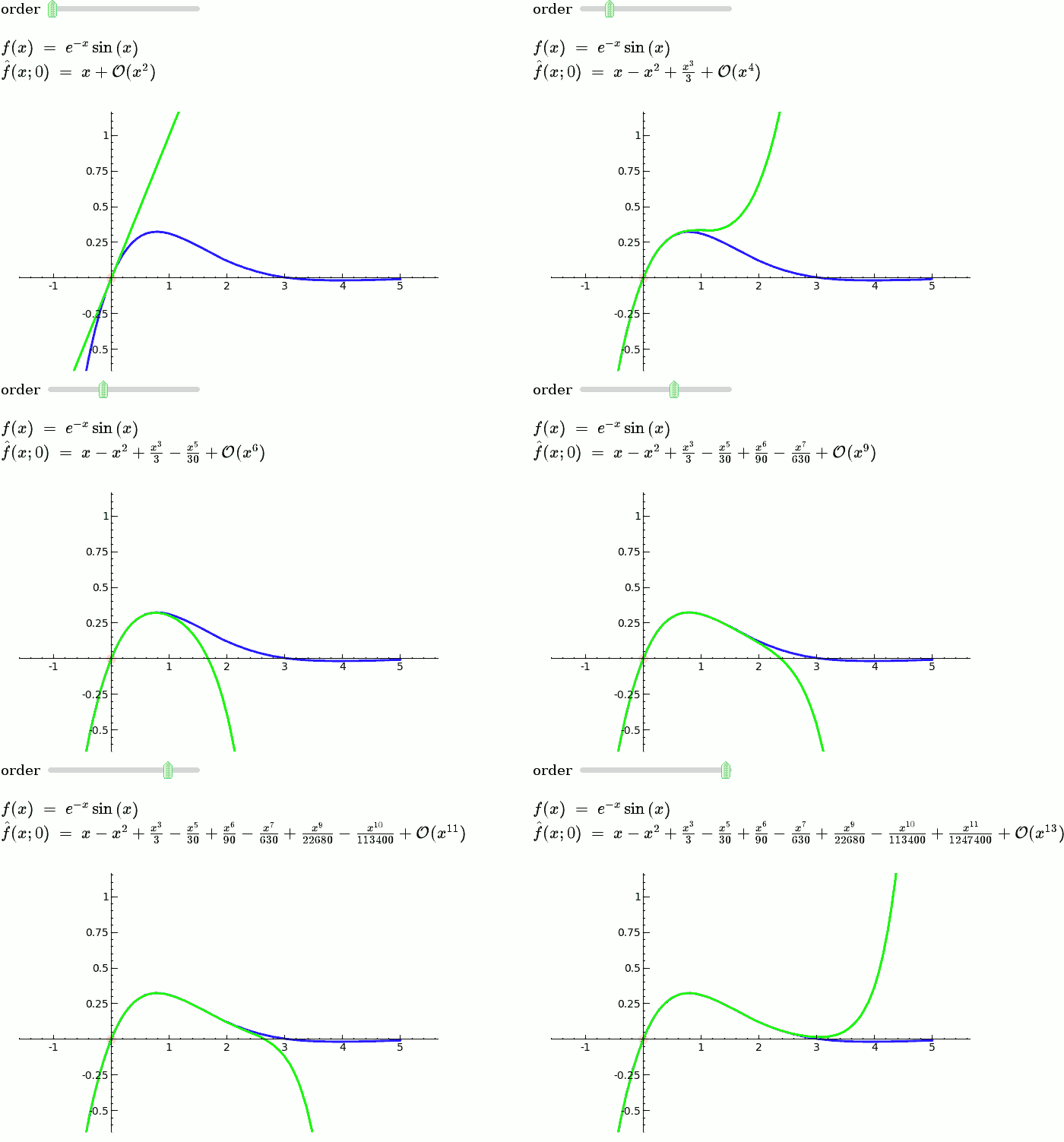
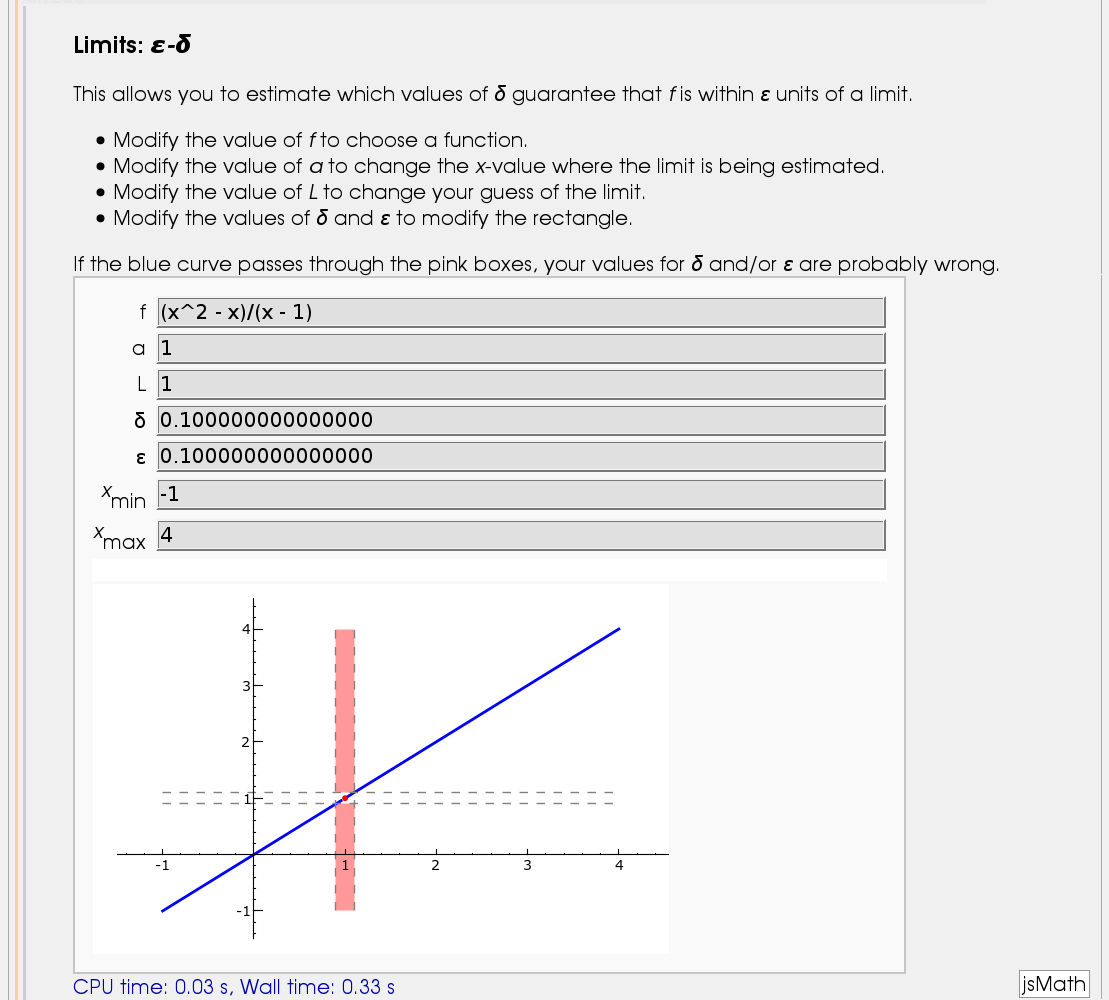
Illustration of the precise definition of a limit
by John Perry
I'll break tradition and put the image first. Apologies if this is Not A Good Thing.
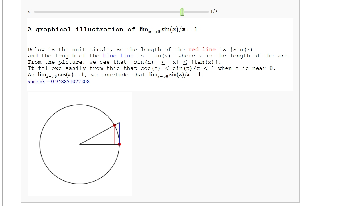
A graphical illustration of sin(x)/x -> 1 as x-> 0
by Wai Yan Pong
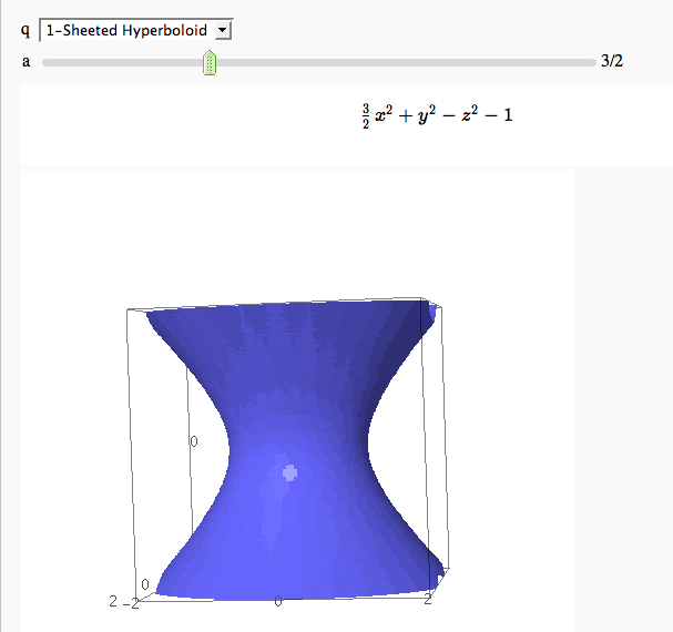
Quadric Surface Plotter
by Marshall Hampton. This is pretty simple, so I encourage people to spruce it up. In particular, it isn't set up to show all possible types of quadrics.
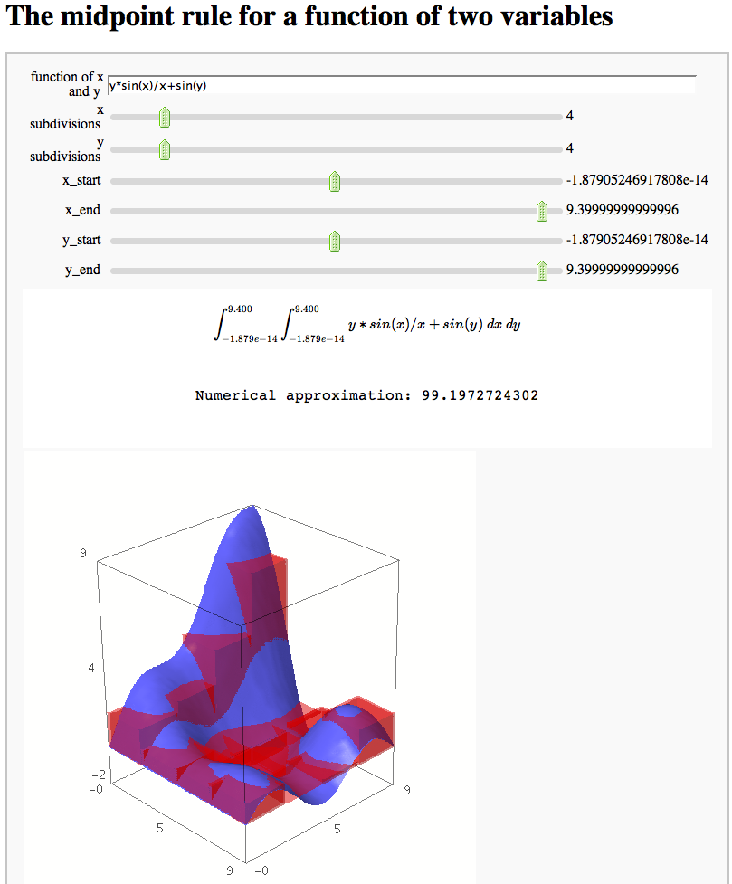
The midpoint rule for numerically integrating a function of two variables
by Marshall Hampton
Gaussian (Legendre) quadrature
by Jason Grout
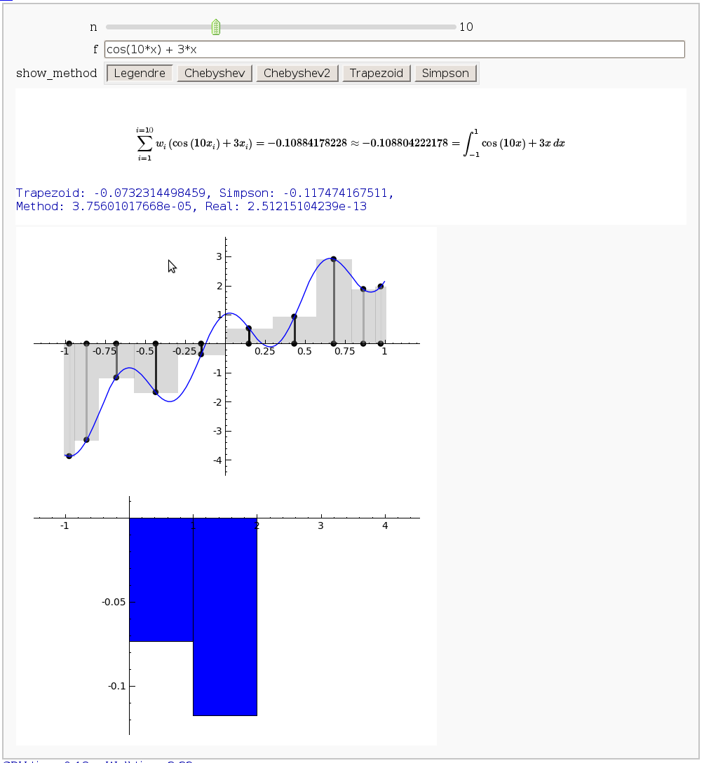
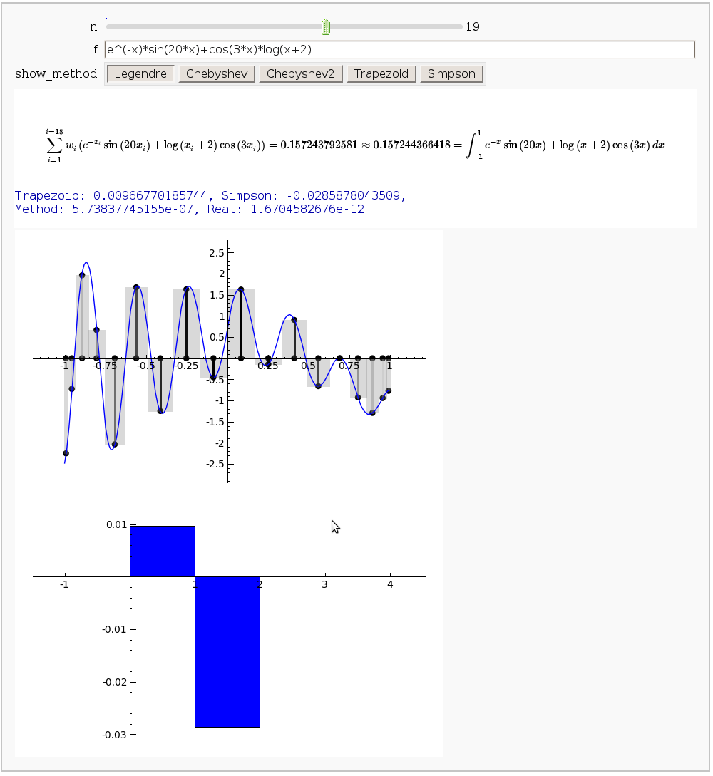
The output shows the points evaluated using Gaussian quadrature (using a weight of 1, so using Legendre polynomials). The vertical bars are shaded to represent the relative weights of the points (darker = more weight). The error in the trapezoid, Simpson, and quadrature methods is both printed out and compared through a bar graph. The "Real" error is the error returned from scipy on the definite integral.
Vector Calculus, 2-D Motion
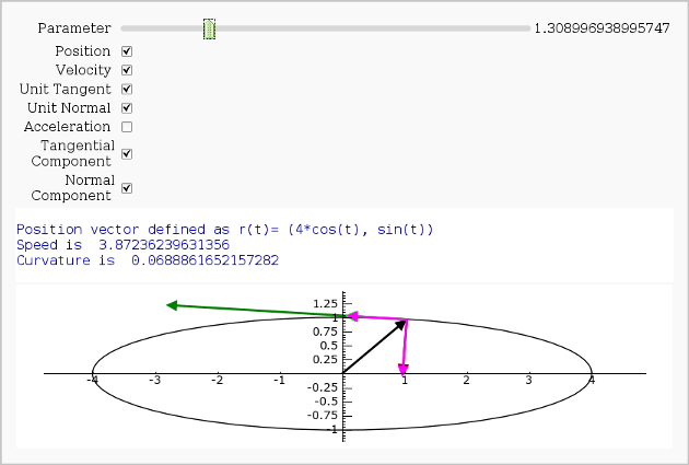
By Rob Beezer
A fast_float() version is available in a worksheet
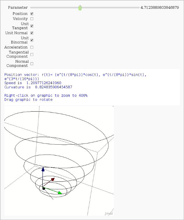
Vector Calculus, 3-D Motion (FIXME)
by Rob Beezer
Available as a worksheet
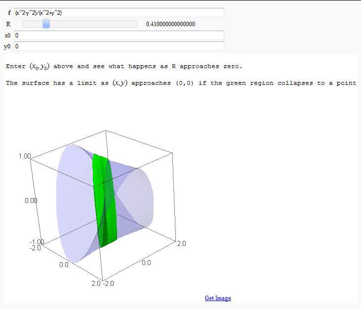
Multivariate Limits by Definition
by John Travis
http://sagenb.mc.edu/home/pub/97/
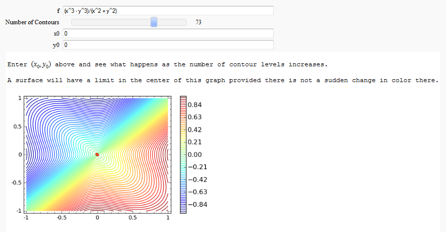
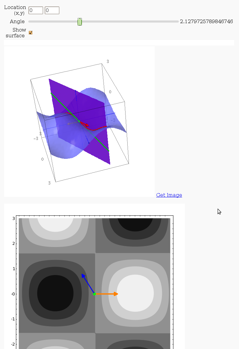
Directional Derivatives
This interact displays graphically a tangent line to a function, illustrating a directional derivative (the slope of the tangent line).
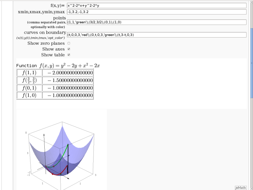
3D graph with points and curves
By Robert Marik
This sagelet is handy when showing local, constrained and absolute maxima and minima in two variables. Available as a worksheet
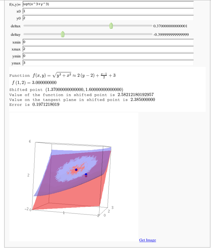
Approximating function in two variables by differential
by Robert Marik
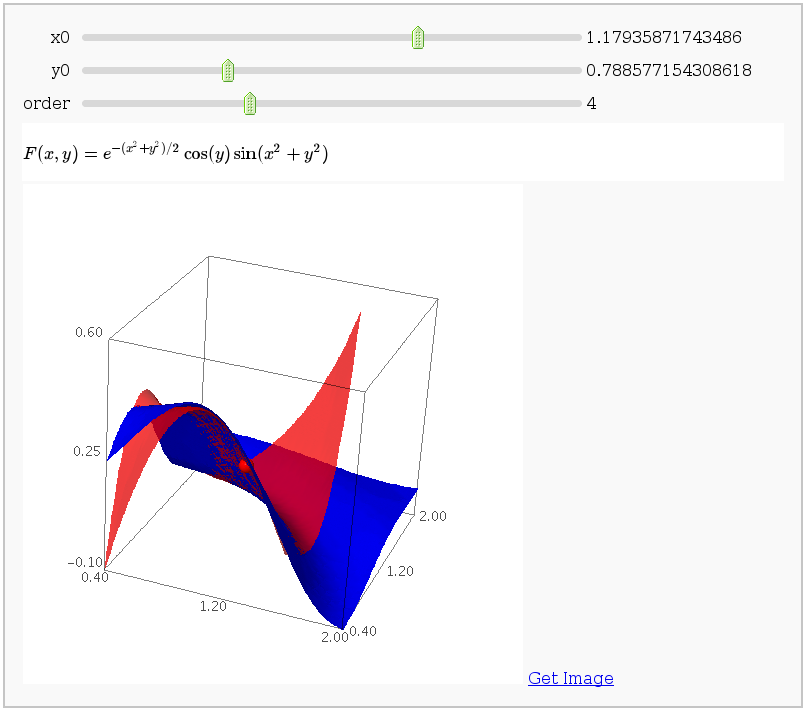
Taylor approximations in two variables
by John Palmieri
This displays the nth order Taylor approximation, for n from 1 to 10, of the function sin(x2 + y2) cos(y) exp(-(x2+y2)/2).
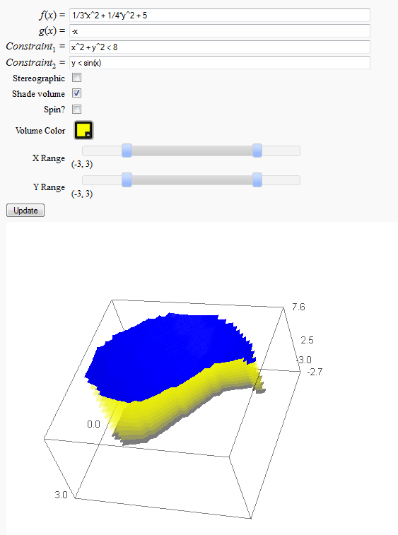
Volumes over non-rectangular domains
by John Travis
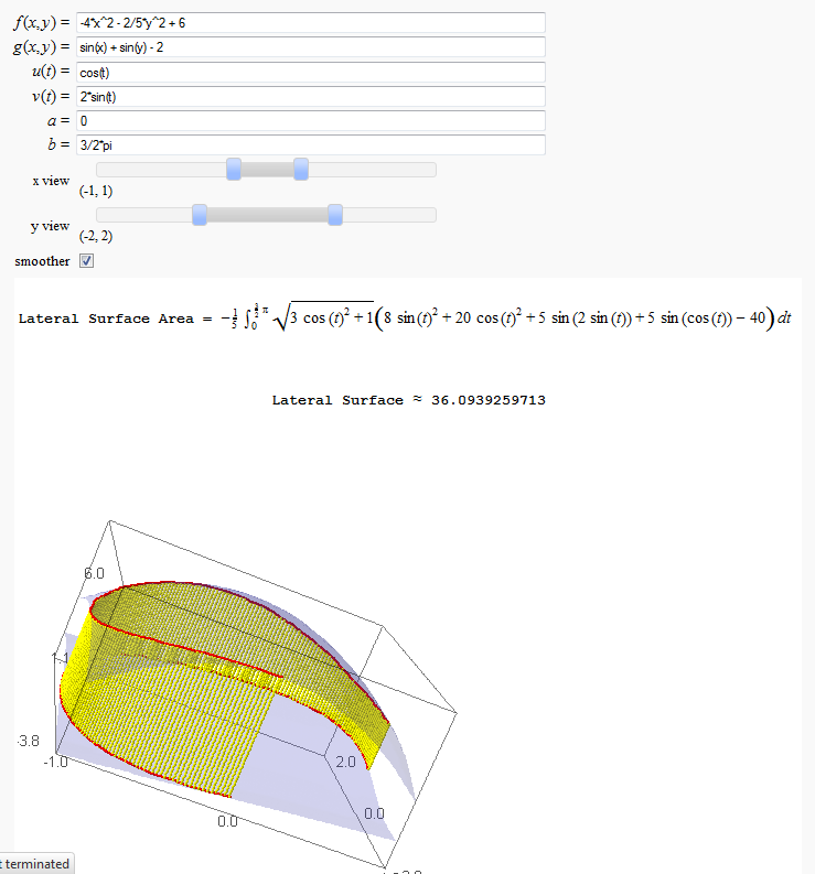
Lateral Surface Area (FIXME in Jupyter)
by John Travis
http://sagenb.mc.edu/home/pub/89/
Parametric surface example (FIXME in Jupyter)
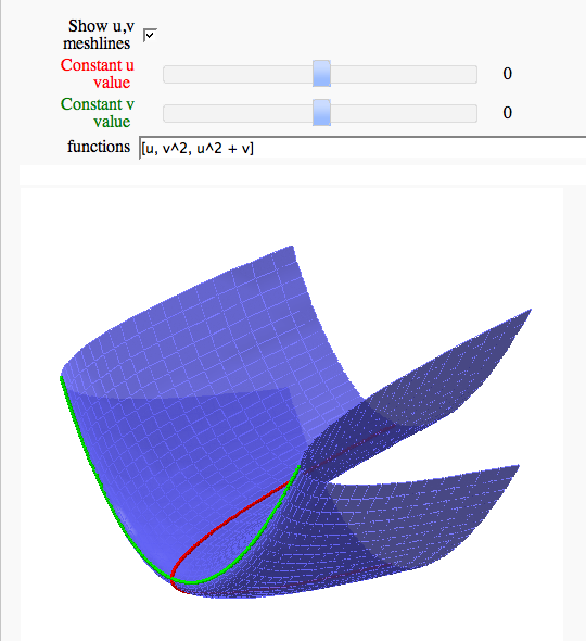
by Marshall Hampton
Line Integrals in 3D Vector Field
by John Travis
