|
Size: 62928
Comment: set homogeneous label format in Illustration of the precise definition of a limit
|
Size: 62984
Comment:
|
| Deletions are marked like this. | Additions are marked like this. |
| Line 27: | Line 27: |
| raise ValueError, "f must have a sign change in the interval (%s,%s)"%(a,b) | raise ValueError("f must have a sign change in the interval (%s,%s)"%(a,b)) |
| Line 33: | Line 33: |
| print "eps = %s"%float(eps) | print("eps = %s" % float(eps)) |
| Line 37: | Line 37: |
| print "f must have opposite sign at the endpoints of the interval" | print("f must have opposite sign at the endpoints of the interval") |
| Line 40: | Line 40: |
| print "root =", c print "f(c) = %r"%f(x=c) print "iterations =", len(intervals) |
print("root =", c) print("f(c) = %r" % f(x=c)) print("iterations =", len(intervals)) |
| Line 69: | Line 69: |
| for i in xrange(maxiter): | for i in range(maxiter): |
| Line 81: | Line 81: |
| print "eps = %s"%float(eps) | print("eps = %s"%float(eps)) |
| Line 83: | Line 83: |
| print "root =", z print "f(c) = %r"%f(x=z) |
print("root = {}".format(z)) print("f(c) = %r" % f(x=z)) |
| Line 86: | Line 86: |
| print "iterations =", n | print("iterations = {}".format(n)) |
| Line 127: | Line 127: |
| print 'Tangent line is y = ' + tanf._repr_() | print('Tangent line is y = ' + tanf._repr_()) |
| Line 155: | Line 155: |
| pretty_print(html('$\int_{a}^{b}{f(x) dx} {\\approx} \sum_i{f(x_i) \Delta x}$')) print "\n\nSage numerical answer: " + str(integral_numerical(func,a,b,max_points = 200)[0]) print "Midpoint estimated answer: " + str(RDF(dx*sum([midys[q] for q in range(n)]))) |
pretty_print(html(r'$\int_{a}^{b}{f(x) dx} {\approx} \sum_i{f(x_i) \Delta x}$')) print("\n\nSage numerical answer: " + str(integral_numerical(func,a,b,max_points = 200)[0])) print("Midpoint estimated answer: " + str(RDF(dx*sum([midys[q] for q in range(n)])))) |
| Line 257: | Line 257: |
| except TypeError, msg: print msg[-200:] print "Unable to make sense of f,g, or a as symbolic expressions." |
except TypeError as msg: print(msg[-200:]) print("Unable to make sense of f,g, or a as symbolic expressions.") |
| Line 446: | Line 446: |
| == Coordinate Transformations (FIXME in Jupyter) == | == Coordinate Transformations == |
| Line 466: | Line 466: |
| u_percent=slider(0,1,0.05,label="<font color='red'>u</font>", default=.7), v_percent=slider(0,1,0.05,label="<font color='blue'>v</font>", default=.7), |
u_percent=slider(0,1,0.05,label="u", default=.7), v_percent=slider(0,1,0.05,label="v", default=.7), |
| Line 497: | Line 497: |
| jacobian=abs(T.diff().det()).simplify_full() | jacobian(u,v)=abs(T.diff().det()).simplify_full() |
| Line 508: | Line 508: |
| pretty_print(table([[uvplot,xyplot]])) | show(graphics_array([uvplot,xyplot])) |
| Line 527: | Line 527: |
| pretty_print(html('$f(x)\;=\;%s$'%latex(f))) pretty_print(html('$\hat{f}(x;%s)\;=\;%s+\mathcal{O}(x^{%s})$'%(x0,latex(ft),order+1))) |
pretty_print(html(r'$f(x)\;=\;%s$'%latex(f))) pretty_print(html(r'$\hat{f}(x;%s)\;=\;%s+\mathcal{O}(x^{%s})$'%(x0,latex(ft),order+1))) |
| Line 549: | Line 549: |
| def delta_epsilon(f = input_box(default=(x^2-x)/(x-1), label=$f$), a=input_box(default=1, label=$a$), L = input_box(default=1, label=$L$), delta=input_box(label=r"$\delta$",default=0.1), epsilon=input_box(label=r"$\varepsilon$",default=0.1), xm=input_box(label=r"$x_{min}$",default=-1), xM=input_box(label=r"$x_{max}$",default=4)): | def delta_epsilon(f = input_box(default=(x^2-x)/(x-1), label="$f$"), a=input_box(default=1, label="$a$"), L = input_box(default=1, label="$L$"), delta=input_box(label=r"$\delta$",default=0.1), epsilon=input_box(label=r"$\varepsilon$",default=0.1), xm=input_box(label=r"$x_{min}$",default=-1), xM=input_box(label=r"$x_{max}$",default=4)): |
| Line 571: | Line 571: |
| pretty_print(html('<h3>A graphical illustration of $\lim_{x -> 0} \sin(x)/x =1$</h3>')) pretty_print(html('Below is the unit circle, so the length of the <font color=red>red line</font> is |sin(x)|')) pretty_print(html('and the length of the <font color=blue>blue line</font> is |tan(x)| where x is the length of the arc.')) pretty_print(html('From the picture, we see that |sin(x)| $\le$ |x| $\le$ |tan(x)|.')) pretty_print(html('It follows easily from this that cos(x) $\le$ sin(x)/x $\le$ 1 when x is near 0.')) pretty_print(html('As $\lim_{x ->0} \cos(x) =1$, we conclude that $\lim_{x -> 0} \sin(x)/x =1$.')) |
pretty_print(html(r'<h3>A graphical illustration of $\lim_{x -> 0} \sin(x)/x =1$</h3>')) pretty_print(html(r'Below is the unit circle, so the length of the <font color=red>red line</font> is |sin(x)|')) pretty_print(html(r'and the length of the <font color=blue>blue line</font> is |tan(x)| where x is the length of the arc.')) pretty_print(html(r'From the picture, we see that |sin(x)| $\le$ |x| $\le$ |tan(x)|.')) pretty_print(html(r'It follows easily from this that cos(x) $\le$ sin(x)/x $\le$ 1 when x is near 0.')) pretty_print(html(r'As $\lim_{x ->0} \cos(x) =1$, we conclude that $\lim_{x -> 0} \sin(x)/x =1$.')) |
| Line 597: | Line 597: |
| def quads(q = selector(quadrics.keys()), a = slider(0,5,1/2,default = 1)): | def quads(q = selector(list(quadrics)), a = slider(0,5,1/2,default = 1)): |
| Line 599: | Line 599: |
| if a==0 or q=='Cone': html('<center>$'+latex(f)+' \ $'+ '(degenerate)</center>') else: html('<center>$'+latex(f)+'$ </center>') |
if a==0 or q=='Cone': pretty_print(latex(f), " (degenerate)") else: pretty_print(latex(f)) |
| Line 628: | Line 628: |
| pretty_print(html("<h1>The midpoint rule for a function of two variables</h1>")) | pretty_print(html(r"<h1>The midpoint rule for a function of two variables</h1>")) |
| Line 643: | Line 643: |
| pretty_print(html("$$\int_{"+str(R16(y_start))+"}^{"+str(R16(y_end))+"} "+ "\int_{"+str(R16(x_start))+"}^{"+str(R16(x_end))+"} "+func+"\ dx \ dy$$")) pretty_print(html('<p style="text-align: center;">Numerical approximation: ' + str(num_approx)+'</p>')) |
pretty_print(html(r"$\int_{"+str(R16(y_start))+r"}^{"+str(R16(y_end))+r"} "+ r"\int_{"+str(R16(x_start))+r"}^{"+str(R16(x_end))+r"} "+latex(SR(func))+r"\ dx \ dy$")) pretty_print(html(r'<p style="text-align: center;">Numerical approximation: ' + str(num_approx)+r'</p>')) |
| Line 660: | Line 660: |
| from numpy import linspace | from numpy import linspace, asanyarray, diff |
| Line 712: | Line 712: |
| y_val = map(scaled_ff,x_val) | y_val = [*map(scaled_ff,x_val)] |
| Line 715: | Line 715: |
| pretty_print(html("$$\sum_{i=1}^{i=%s}w_i\left(%s\\right)= %s\\approx %s =\int_{-1}^{1}%s \,dx$$"%(n, | pretty_print(html(r"$$\sum_{i=1}^{i=%s}w_i\left(%s\right)= %s\approx %s =\int_{-1}^{1}%s \,dx$$"%(n, |
| Line 718: | Line 718: |
| print "Trapezoid: %s, Simpson: %s, \nMethod: %s, Real: %s"%tuple(error_data) | print("Trapezoid: %s, Simpson: %s, \nMethod: %s, Real: %s" % tuple(error_data)) |
| Line 756: | Line 756: |
| path = parametric_plot( position(t).list(), (t, start, stop), color = "black" ) | path = parametric_plot( position.list(), (t, start, stop), color = "black" ) |
| Line 760: | Line 760: |
| velocity = derivative(position(t), t) acceleration = derivative(velocity(t), t) |
velocity = derivative(position, t) acceleration = derivative(velocity, t) |
| Line 765: | Line 765: |
| dT = derivative(tangent(t), t) | dT = derivative(tangent, t) |
| Line 786: | Line 786: |
| pos_tzero = position(t0) | pos_tzero = position(t=t0) |
| Line 790: | Line 790: |
| speed_component = speed(t0) tangent_component = speed_deriv(t0) normal_component = sqrt( acceleration(t0).norm()^2 - tangent_component^2 ) |
speed_component = speed(t=t0) tangent_component = speed_deriv(t=t0) normal_component = sqrt( acceleration(t=t0).norm()^2 - tangent_component^2 ) |
| Line 798: | Line 798: |
| tan = arrow(pos_tzero, pos_tzero + tangent(t0), rgbcolor=(0,1,0) ) vel = arrow(pos_tzero, pos_tzero + velocity(t0), rgbcolor=(0,0.5,0)) nor = arrow(pos_tzero, pos_tzero + normal(t0), rgbcolor=(0.5,0,0)) acc = arrow(pos_tzero, pos_tzero + acceleration(t0), rgbcolor=(1,0,1)) tancomp = arrow(pos_tzero, pos_tzero + tangent_component*tangent(t0), rgbcolor=(1,0,1) ) norcomp = arrow(pos_tzero, pos_tzero + normal_component*normal(t0), rgbcolor=(1,0,1)) |
tan = arrow(pos_tzero, pos_tzero + tangent(t=t0), rgbcolor=(0,1,0) ) vel = arrow(pos_tzero, pos_tzero + velocity(t=t0), rgbcolor=(0,0.5,0)) nor = arrow(pos_tzero, pos_tzero + normal(t=t0), rgbcolor=(0.5,0,0)) acc = arrow(pos_tzero, pos_tzero + acceleration(t=t0), rgbcolor=(1,0,1)) tancomp = arrow(pos_tzero, pos_tzero + tangent_component*tangent(t=t0), rgbcolor=(1,0,1) ) norcomp = arrow(pos_tzero, pos_tzero + normal_component*normal(t=t0), rgbcolor=(1,0,1)) |
| Line 825: | Line 825: |
| print "Position vector defined as r(t)=", position(t) print "Speed is ", N(speed(t0)) print "Curvature is ", N(curvature) |
print("Position vector defined as r(t)={}".format(position)) print("Speed is {}".format(N(speed(t=t0)))) print("Curvature is {}".format(N(curvature))) |
| Line 836: | Line 836: |
| == Vector Calculus, 3-D Motion (FIXME) == | == Vector Calculus, 3-D Motion == |
| Line 857: | Line 857: |
| assume(t, 'real') | |
| Line 874: | Line 875: |
| path = parametric_plot3d( position(t).list(), (t, start, stop), color = "black" ) | path = parametric_plot3d( position.list(), (t, start, stop), color = "black" ) |
| Line 878: | Line 879: |
| velocity = derivative( position(t), t) acceleration = derivative(velocity(t), t) |
velocity = derivative( position, t) acceleration = derivative(velocity, t) |
| Line 883: | Line 884: |
| dT = derivative(tangent(t), t) | dT = derivative(tangent, t) |
| Line 886: | Line 887: |
| ## dB = derivative(binormal(t), t) | ## dB = derivative(binormal, t) |
| Line 907: | Line 908: |
| pos_tzero = position(t0) | pos_tzero = position(t=t0) |
| Line 911: | Line 912: |
| speed_component = speed(t0) tangent_component = speed_deriv(t0) normal_component = sqrt( acceleration(t0).norm()^2 - tangent_component^2 ) |
speed_component = speed(t=t0) tangent_component = speed_deriv(t=t0) normal_component = sqrt( acceleration(t=t0).norm()^2 - tangent_component^2 ) |
| Line 920: | Line 921: |
| tan = arrow3d(pos_tzero, pos_tzero + tangent(t0), rgbcolor=(0,1,0) ) vel = arrow3d(pos_tzero, pos_tzero + velocity(t0), rgbcolor=(0,0.5,0)) nor = arrow3d(pos_tzero, pos_tzero + normal(t0), rgbcolor=(0.5,0,0)) bin = arrow3d(pos_tzero, pos_tzero + binormal(t0), rgbcolor=(0,0,0.5)) acc = arrow3d(pos_tzero, pos_tzero + acceleration(t0), rgbcolor=(1,0,1)) tancomp = arrow3d(pos_tzero, pos_tzero + tangent_component*tangent(t0), rgbcolor=(1,0,1) ) norcomp = arrow3d(pos_tzero, pos_tzero + normal_component*normal(t0), rgbcolor=(1,0,1)) |
tan = arrow3d(pos_tzero, pos_tzero + tangent(t=t0), rgbcolor=(0,1,0) ) vel = arrow3d(pos_tzero, pos_tzero + velocity(t=t0), rgbcolor=(0,0.5,0)) nor = arrow3d(pos_tzero, pos_tzero + normal(t=t0), rgbcolor=(0.5,0,0)) bin = arrow3d(pos_tzero, pos_tzero + binormal(t=t0), rgbcolor=(0,0,0.5)) acc = arrow3d(pos_tzero, pos_tzero + acceleration(t=t0), rgbcolor=(1,0,1)) tancomp = arrow3d(pos_tzero, pos_tzero + tangent_component*tangent(t=t0), rgbcolor=(1,0,1) ) norcomp = arrow3d(pos_tzero, pos_tzero + normal_component*normal(t=t0), rgbcolor=(1,0,1)) |
| Line 950: | Line 951: |
| print "Position vector: r(t)=", position(t) print "Speed is ", N(speed(t0)) print "Curvature is ", N(curvature) ## print "Torsion is ", N(torsion) print "Right-click on graphic to zoom to 400%" print "Drag graphic to rotate" |
print("Position vector: r(t)=", position) print("Speed is ", N(speed(t=t0))) print("Curvature is ", N(curvature)) ## print("Torsion is ", N(torsion)) print() print("Right-click on graphic to zoom to 400%") print("Drag graphic to rotate") |
| Line 1032: | Line 1033: |
| pretty_print(html('\n<center><font color="red">$\lim_{(x,?)\\rightarrow(x_0,y_0)} f(x,y) =%s$</font>'%str(limit_x)+' and <font color="red">$\lim_{(?,y)\\rightarrow(x_0,y_0)} f(x,y) =%s$</font></center>'%str(limit_y))) | pretty_print(html(r'<center><font color="red">$\lim_{(x,?)\rightarrow(x_0,y_0)} f(x,y) =%s$</font>'%str(limit_x)+r' and <font color="red">$\lim_{(?,y)\rightarrow(x_0,y_0)} f(x,y) =%s$</font></center>'%str(limit_y))) |
| Line 1251: | Line 1252: |
| order=(1..10)): | order=[1..10]): |
Sage Interactions - Calculus
goto interact main page
Contents
-
Sage Interactions - Calculus
- Root Finding Using Bisection
- Newton's Method
- A contour map and 3d plot of two inverse distance functions
- A simple tangent line grapher
- Numerical integrals with the midpoint rule
- Numerical integrals with various rules
- Some polar parametric curves
- Function tool
- Newton-Raphson Root Finding
- Coordinate Transformations
- Taylor Series
- Illustration of the precise definition of a limit
- A graphical illustration of sin(x)/x -> 1 as x-> 0
- Quadric Surface Plotter
- The midpoint rule for numerically integrating a function of two variables
- Gaussian (Legendre) quadrature
- Vector Calculus, 2-D Motion
- Vector Calculus, 3-D Motion
- Multivariate Limits by Definition
- Directional Derivatives
- 3D graph with points and curves
- Approximating function in two variables by differential
- Taylor approximations in two variables
- Volumes over non-rectangular domains
- Lateral Surface Area (FIXME in Jupyter)
- Parametric surface example (FIXME in Jupyter)
- Line Integrals in 3D Vector Field
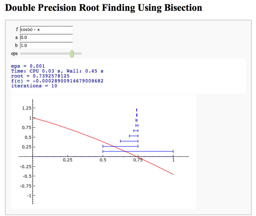
Root Finding Using Bisection
by William Stein
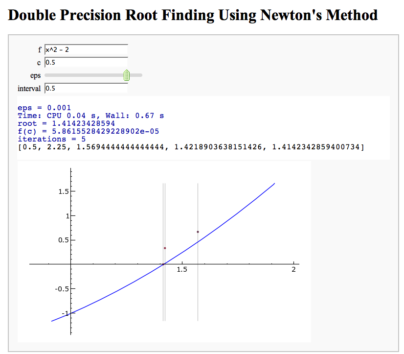
Newton's Method
Note that there is a more complicated Newton's method below.
by William Stein
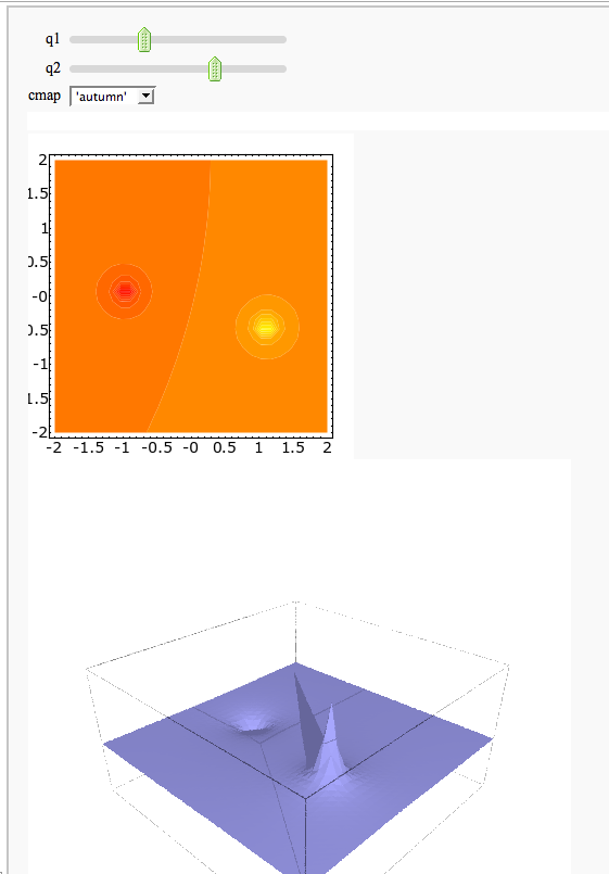
A contour map and 3d plot of two inverse distance functions
by William Stein
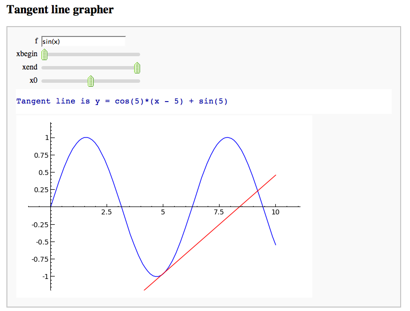
A simple tangent line grapher
by Marshall Hampton
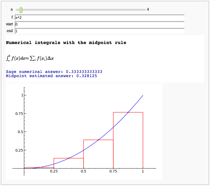
Numerical integrals with the midpoint rule
by Marshall Hampton
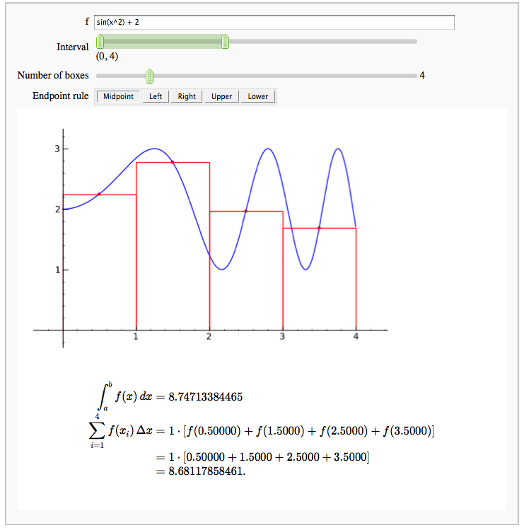
Numerical integrals with various rules
by Nick Alexander (based on the work of Marshall Hampton)
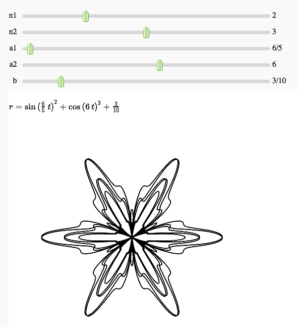
Some polar parametric curves
by Marshall Hampton. This is not very general, but could be modified to show other families of polar curves.
Function tool
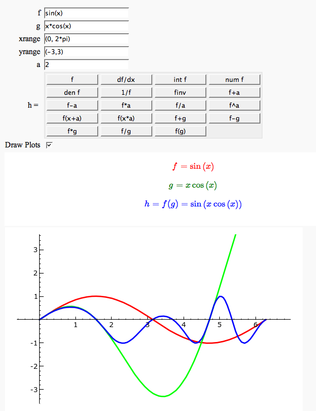
Enter symbolic functions f, g, and a, a range, then click the appropriate button to compute and plot some combination of f, g, and a along with f and g. This is inspired by the Matlab funtool GUI.
Newton-Raphson Root Finding
by Neal Holtz
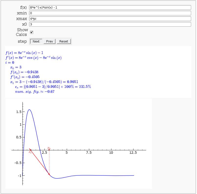
This allows user to display the Newton-Raphson procedure one step at a time. It uses the heuristic that, if any of the values of the controls change, then the procedure should be re-started, else it should be continued.
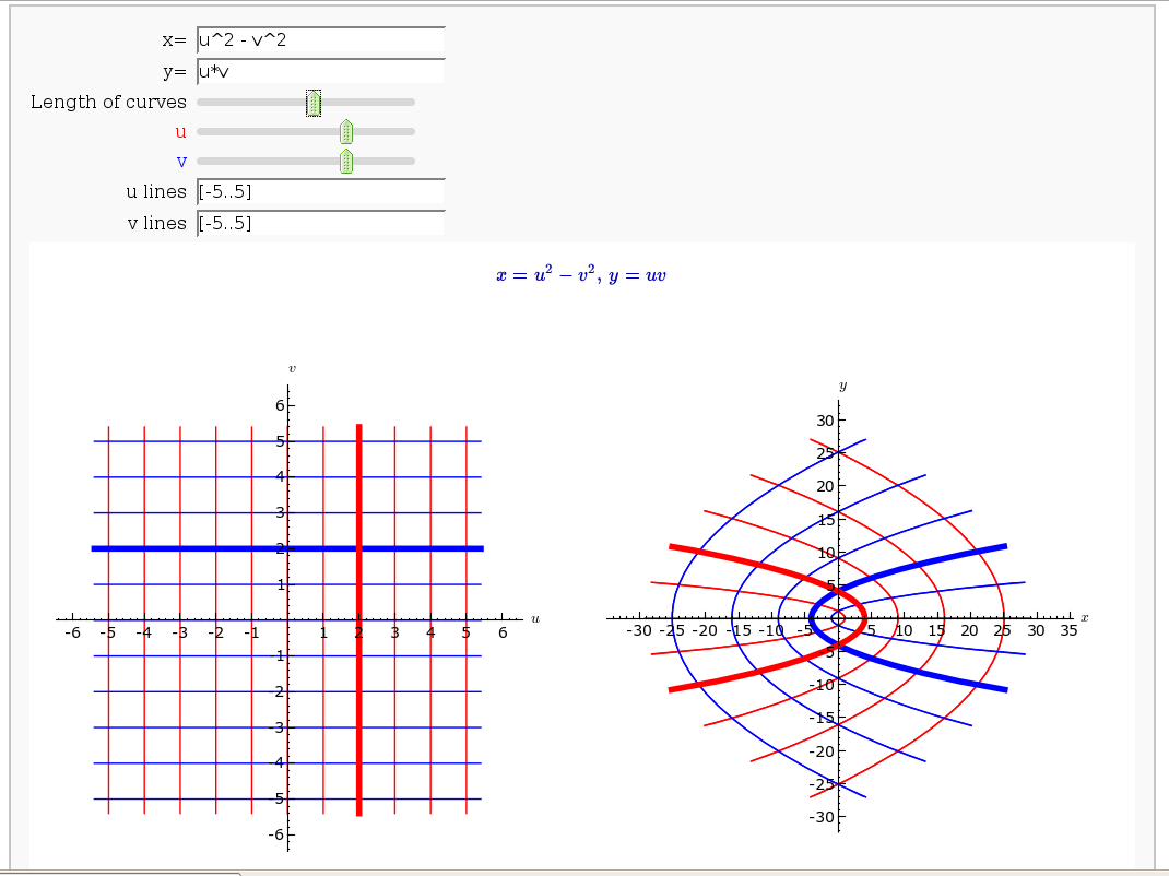
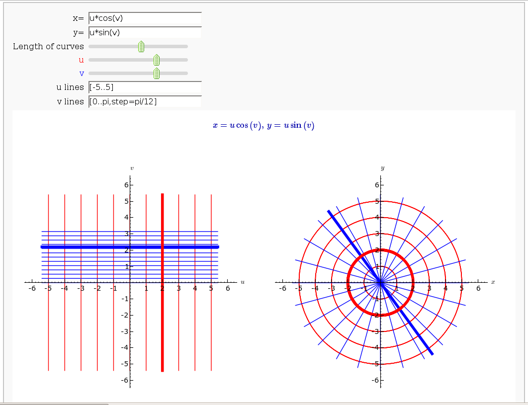
Coordinate Transformations
by Jason Grout
Taylor Series
by Harald Schilly
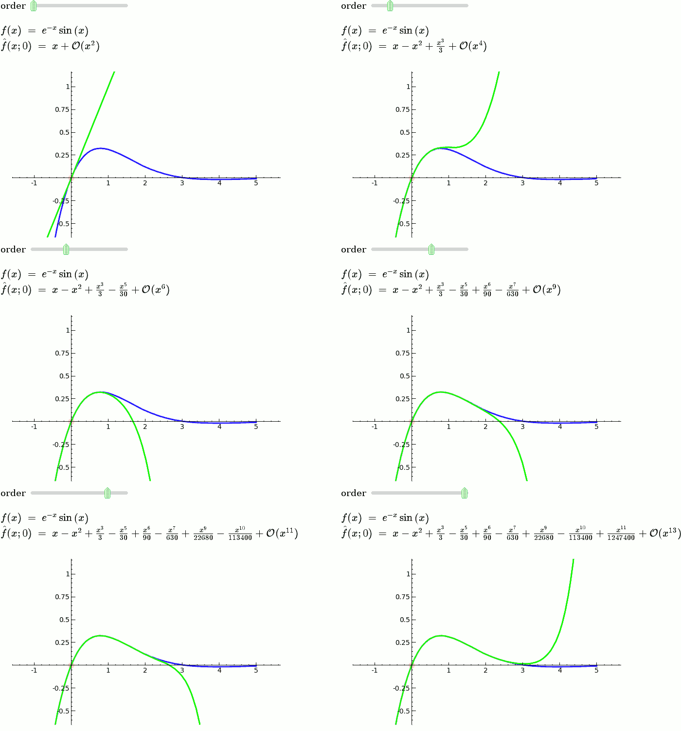
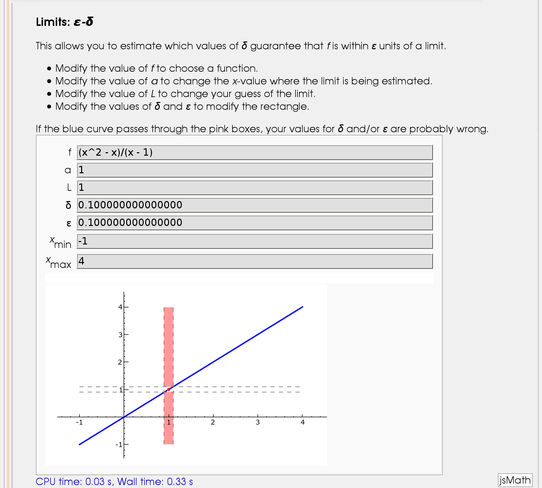
Illustration of the precise definition of a limit
by John Perry
I'll break tradition and put the image first. Apologies if this is Not A Good Thing.
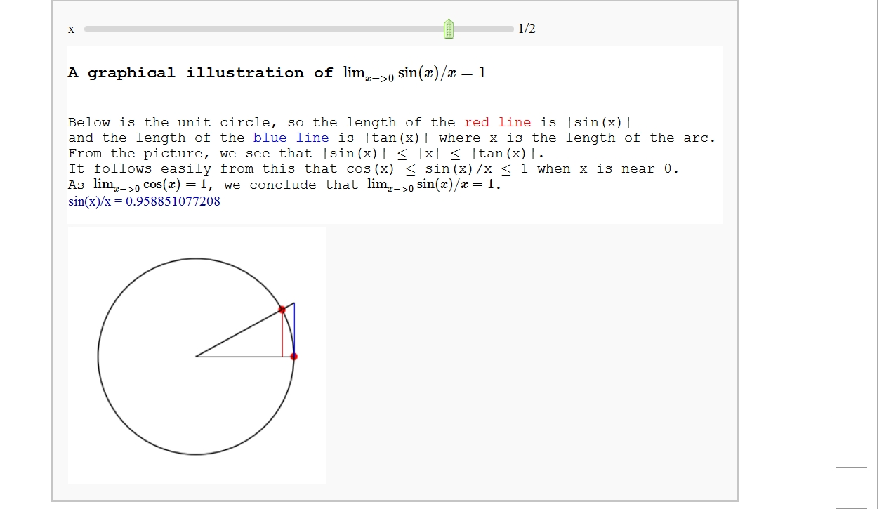
A graphical illustration of sin(x)/x -> 1 as x-> 0
by Wai Yan Pong
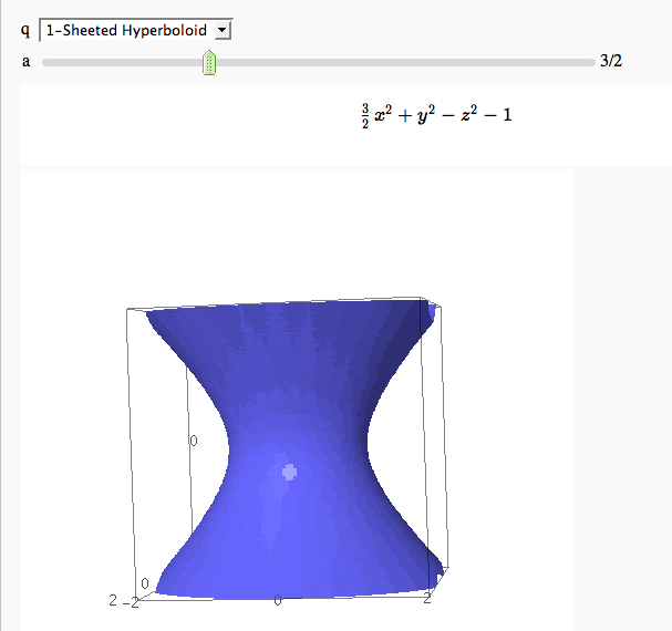
Quadric Surface Plotter
by Marshall Hampton. This is pretty simple, so I encourage people to spruce it up. In particular, it isn't set up to show all possible types of quadrics.
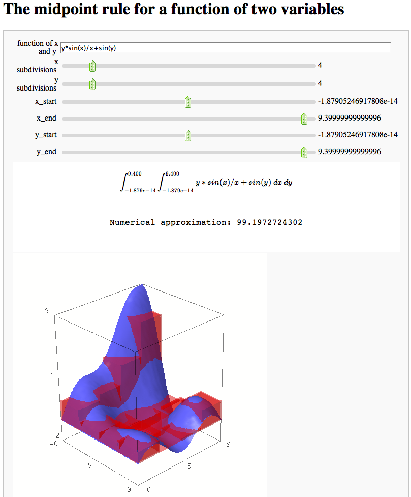
The midpoint rule for numerically integrating a function of two variables
by Marshall Hampton
Gaussian (Legendre) quadrature
by Jason Grout
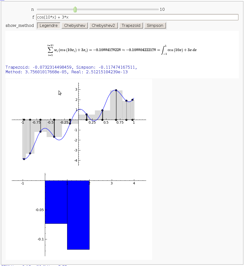
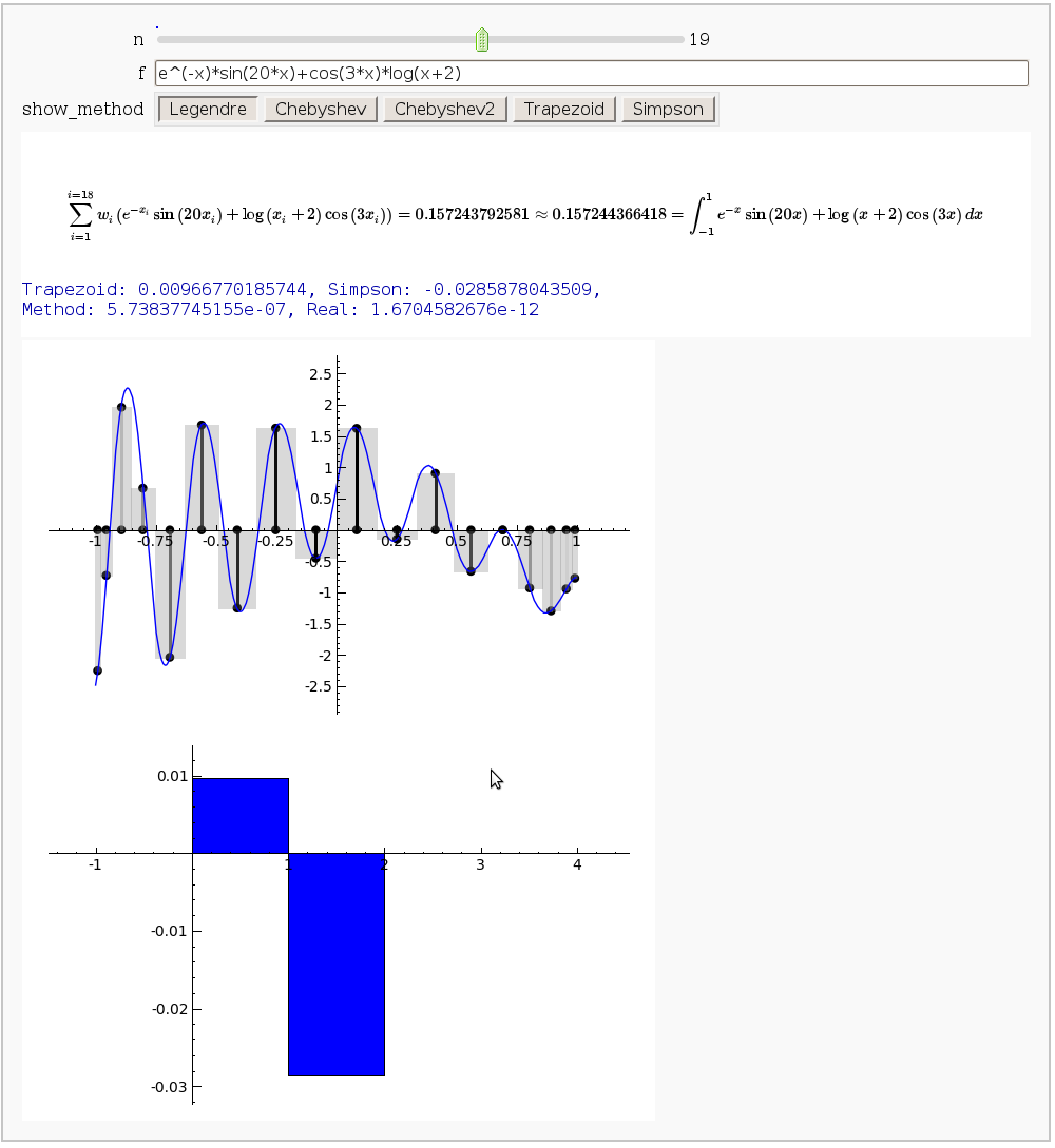
The output shows the points evaluated using Gaussian quadrature (using a weight of 1, so using Legendre polynomials). The vertical bars are shaded to represent the relative weights of the points (darker = more weight). The error in the trapezoid, Simpson, and quadrature methods is both printed out and compared through a bar graph. The "Real" error is the error returned from scipy on the definite integral.
Vector Calculus, 2-D Motion
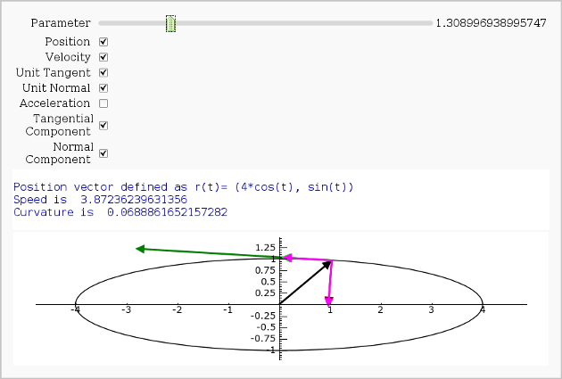
By Rob Beezer
A fast_float() version is available in a worksheet
Vector Calculus, 3-D Motion
by Rob Beezer
Available as a worksheet
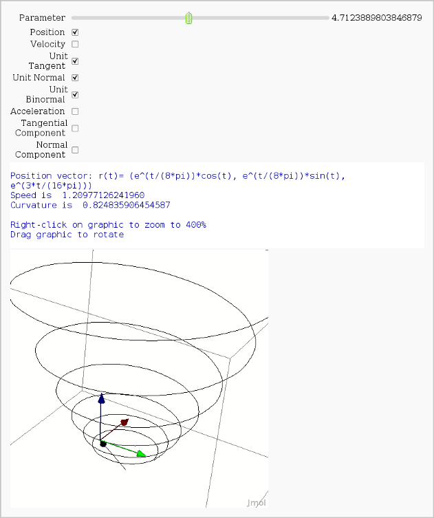
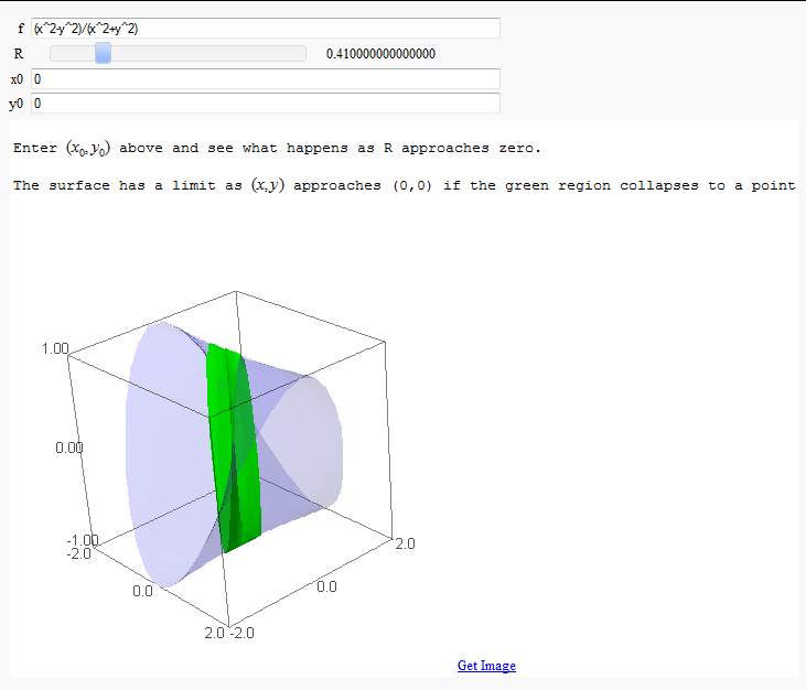
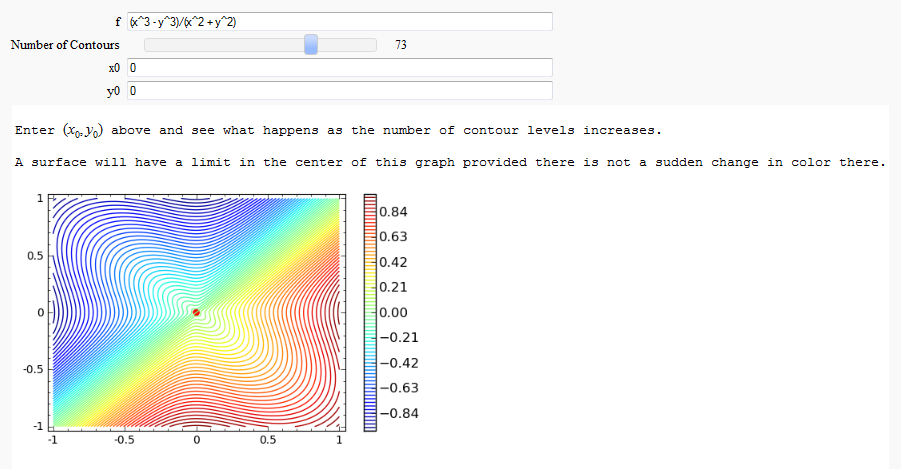
Multivariate Limits by Definition
by John Travis
http://sagenb.mc.edu/home/pub/97/
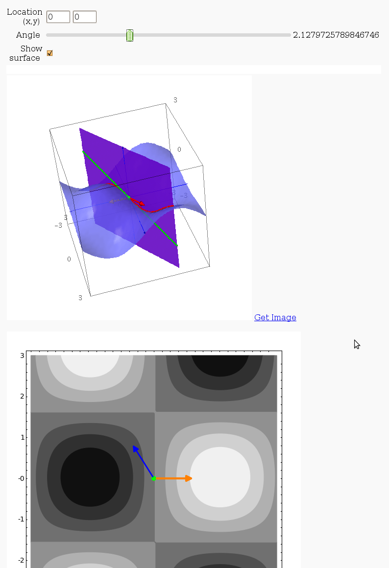
Directional Derivatives
This interact displays graphically a tangent line to a function, illustrating a directional derivative (the slope of the tangent line).
3D graph with points and curves
By Robert Marik
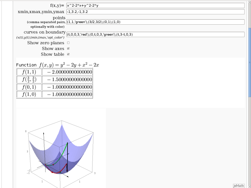
This sagelet is handy when showing local, constrained and absolute maxima and minima in two variables. Available as a worksheet
Approximating function in two variables by differential
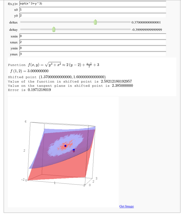
by Robert Marik
Taylor approximations in two variables
by John Palmieri
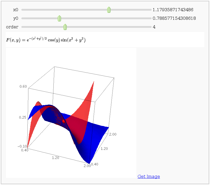
This displays the nth order Taylor approximation, for n from 1 to 10, of the function sin(x2 + y2) cos(y) exp(-(x2+y2)/2).
Volumes over non-rectangular domains
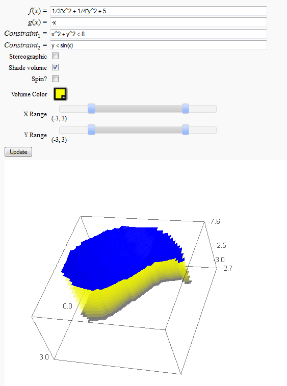
by John Travis
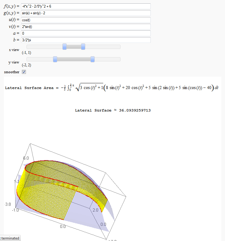
Lateral Surface Area (FIXME in Jupyter)
by John Travis
http://sagenb.mc.edu/home/pub/89/
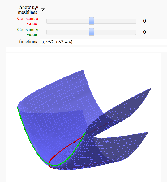
Parametric surface example (FIXME in Jupyter)
by Marshall Hampton
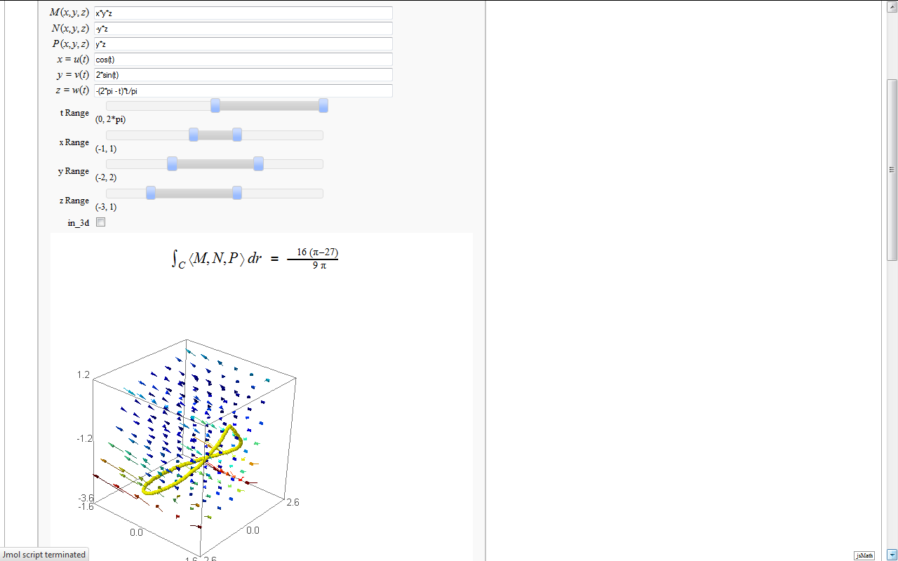
Line Integrals in 3D Vector Field
by John Travis
