|
Size: 30478
Comment:
|
Size: 30348
Comment: fixed Continued Fraction Plotter, more or less
|
| Deletions are marked like this. | Additions are marked like this. |
| Line 51: | Line 51: |
| g += line([(j*2-len(cur),-i), ((k*2)-len(rows[i-1]),-i+1)], | g += line([(j*2-len(cur),-i), ((k*2)-len(rows[i-1]),-i+1)], |
| Line 101: | Line 101: |
| REFERENCES: | REFERENCES: |
| Line 106: | Line 106: |
| Weisstein, Eric W. "Prime-Generating Polynomial." From MathWorld--A Wolfram Web Resource. http://mathworld.wolfram.com/Prime-GeneratingPolynomial.html | Weisstein, Eric W. "Prime-Generating Polynomial." From MathWorld--A Wolfram Web Resource. http://mathworld.wolfram.com/Prime-GeneratingPolynomial.html |
| Line 114: | Line 114: |
| elif y<0 and -x >= y and y<x: return 4*(y+1)^2 -11*(y+1) + (start+7) +x | elif y<0 and -x >= y and y<x: return 4*(y+1)^2 -11*(y+1) + (start+7) +x |
| Line 117: | Line 117: |
| #Takes in an n and the start value of the spiral and gives its (x,y) coordinate | #Takes in an n and the start value of the spiral and gives its (x,y) coordinate |
| Line 119: | Line 119: |
| num = num - start +1 | num = num - start +1 |
| Line 121: | Line 121: |
| top = ceil(sqrt(num)) | top = ceil(sqrt(num)) |
| Line 126: | Line 126: |
| else: | else: |
| Line 133: | Line 133: |
| else: | else: |
| Line 145: | Line 145: |
| N = M.copy() | N = copy(M) |
| Line 149: | Line 149: |
| #These functions return an int based on where the t is located in the spiral |
#These functions return an int based on where the t is located in the spiral |
| Line 162: | Line 162: |
| if n !=0: x_cord, y_cord = find_xy(n, start) #Overrides the user given x and y coordinates | if n !=0: x_cord, y_cord = find_xy(n, start) #Overrides the user given x and y coordinates |
| Line 170: | Line 170: |
| Line 173: | Line 173: |
| if show_lines: for t in [(-size-1)..size+1]: |
if show_lines: for t in [(-size-1)..size+1]: |
| Line 176: | Line 176: |
| if m.is_pseudoprime(): main_list.add(m) | if m.is_pseudoprime(): main_list.add(m) |
| Line 181: | Line 181: |
| #This for loop changes the matrix by spiraling out from the center and changing each entry as it goes. It is faster than the find_xy function above. | #This for loop changes the matrix by spiraling out from the center and changing each entry as it goes. It is faster than the find_xy function above. |
| Line 186: | Line 186: |
| else: x-=1 | else: x-=1 |
| Line 188: | Line 188: |
| elif county < overcount: |
elif county < overcount: |
| Line 191: | Line 191: |
| else: y-=1 | else: y-=1 |
| Line 193: | Line 193: |
| else: | else: |
| Line 199: | Line 199: |
| if not invert and num in main_list: |
if not invert and num in main_list: |
| Line 207: | Line 207: |
| if n != 0: |
if n != 0: |
| Line 224: | Line 224: |
| else: | else: |
| Line 235: | Line 235: |
| def polar_prime_spiral(start=1, end=2000, show_factors = false, highlight_primes = false, show_curves=true, n = 0): #For more information about the factors in the spiral, visit http://www.dcs.gla.ac.uk/~jhw/spirals/index.html by John Williamson. |
def polar_prime_spiral(start=1, end=2000, show_factors = false, highlight_primes = false, show_curves=true, n = 0): #For more information about the factors in the spiral, visit http://www.dcs.gla.ac.uk/~jhw/spirals/index.html by John Williamson. |
| Line 243: | Line 243: |
| Line 251: | Line 251: |
| R = points(list2, alpha = .1) #Faded Composites else: |
R = points(list2, alpha = .1) #Faded Composites else: |
| Line 259: | Line 259: |
| R=points(list2, hue = .1, pointsize = p_size) |
R=points(list2, hue = .1, pointsize = p_size) |
| Line 263: | Line 263: |
| Line 270: | Line 270: |
| Q = plot(W1+W2+W3+W4, alpha = .1) | Q = plot(W1+W2+W3+W4, alpha = .1) |
| Line 273: | Line 273: |
| if show_curves: | if show_curves: |
| Line 278: | Line 278: |
| if n > (floor(sqrt(n)))^2 and n <= (floor(sqrt(n)))^2 + floor(sqrt(n)): | if n > (floor(sqrt(n)))^2 and n <= (floor(sqrt(n)))^2 + floor(sqrt(n)): |
| Line 281: | Line 281: |
| else: | else: |
| Line 286: | Line 286: |
| def g(m): return (a*m^2+b*m+c); | def g(m): return (a*m^2+b*m+c); |
| Line 292: | Line 292: |
| c= c2; | c= c2; |
| Line 305: | Line 305: |
| == Computing modular forms FIXME == | == Computing modular forms == |
| Line 308: | Line 308: |
| j = 0 @interact def _(N=[1..100], k=selector([2,4,..,12],nrows=1), prec=(3..40), |
@interact def _(N=[1..100], k=selector([2,4,..,12],nrows=1), prec=(3..40), |
| Line 313: | Line 312: |
| print j; global j; j += 1 | |
| Line 340: | Line 338: |
| == A Charpoly and Hecke Operator Graph FIXME == | == A Charpoly and Hecke Operator Graph == |
| Line 351: | Line 349: |
| G = Graph(T, multiedges=True, loops=not three_d) | G = DiGraph(T, multiedges=not three_d) if three_d: G.remove_loops() |
| Line 472: | Line 472: |
| MP += line([(i,0),(i,r)], rgbcolor='black') | MP += line([(i,0),(i,r)], rgbcolor='black') |
| Line 553: | Line 553: |
| S += point(e_pt,pointsize=50, rgbcolor='red') | S += point(e_pt,pointsize=50, rgbcolor='red') |
| Line 556: | Line 556: |
| S += point(f_gs_pt,pointsize=75, rgbcolor='black') | S += point(f_gs_pt,pointsize=75, rgbcolor='black') |
| Line 561: | Line 561: |
| S += text('$J(%s,%s) = %s$'%(latex2(e),latex2(f),latex(js)), | S += text('$J(%s,%s) = %s$'%(latex2(e),latex2(f),latex(js)), |
| Line 629: | Line 629: |
| S = circle((0,0),1,rgbcolor='yellow') \ + line([e_pt,e_gs_pt], rgbcolor='red', thickness=4) \ + line([f_pt,f_gs_pt], rgbcolor='blue', thickness=3) \ + line([ef_pt,ef_gs_pt], rgbcolor='purple',thickness=2) \ + point(e_pt,pointsize=50, rgbcolor='red') \ + point(f_pt,pointsize=50, rgbcolor='blue') \ + point(ef_pt,pointsize=50,rgbcolor='purple') \ + point(f_gs_pt,pointsize=75, rgbcolor='black') \ + point(e_gs_pt,pointsize=75, rgbcolor='black') \ + point(ef_gs_pt,pointsize=75, rgbcolor='black') \ + point(js_pt,pointsize=100,rgbcolor='green') |
S = circle((0,0),1,rgbcolor='yellow') S += line([e_pt,e_gs_pt], rgbcolor='red', thickness=4) S += line([f_pt,f_gs_pt], rgbcolor='blue', thickness=3) S += line([ef_pt,ef_gs_pt], rgbcolor='purple',thickness=2) S += point(e_pt,pointsize=50, rgbcolor='red') S += point(f_pt,pointsize=50, rgbcolor='blue') S += point(ef_pt,pointsize=50,rgbcolor='purple') S += point(f_gs_pt,pointsize=75, rgbcolor='black') S += point(e_gs_pt,pointsize=75, rgbcolor='black') S += point(ef_gs_pt,pointsize=75, rgbcolor='black') S += point(js_pt,pointsize=100,rgbcolor='green') |
| Line 641: | Line 641: |
| S += text('$J(%s,%s) = %s$'%(latex2(e),latex2(f),latex(js)), \ | S += text('$J(%s,%s) = %s$'%(latex2(e),latex2(f),latex(js)), |
| Line 653: | Line 653: |
| ga[i].save('j%d.PNG'%i,figsize=4,aspect_ratio=1, \ | ga[i].save('j%d.png'%i,figsize=4,aspect_ratio=1, |
| Line 659: | Line 659: |
| html('<table bgcolor=lightgrey cellpadding=2>') | s='<table bgcolor=lightgrey cellpadding=2>' |
| Line 661: | Line 661: |
| html('<tr><td align="center"><img src="cell://j%d.PNG"></td>'%(2*i)) html('<td align="center"><img src="cell://j%d.PNG"></td></tr>'%(2*i+1)) html('</table>') }}} |
s+='<tr><td align="center"><img src="cell://j%d.png"></td>'%(2*i) s+='<td align="center"><img src="cell://j%d.png"></td></tr>'%(2*i+1) s+='</table>' html(s)}}} |
| Line 678: | Line 678: |
| else: | else: |
| Line 685: | Line 685: |
def line_from_curve_points(E,P,Q,style='-',rgb=(1,0,0),length=25): """ P,Q two points on an elliptic curve. Output is a graphic representation of the straight line intersecting with P,Q. """ # The function tangent to P=Q on E if P == Q: if P[2]==0: return line([(1,-length),(1,length)],linestyle=style,rgbcolor=rgb) else: # Compute slope of the curve E in P l=-(3*P[0]^2 + 2*E.a2()*P[0] + E.a4() - E.a1()*P[1])/((-2)*P[1] - E.a1()*P[0] - E.a3()) f(x) = l * (x - P[0]) + P[1] return plot(f(x),-length,length,linestyle=style,rgbcolor=rgb) # Trivial case of P != R where P=O or R=O then we get the vertical line from the other point elif P[2] == 0: return line([(Q[0],-length),(Q[0],length)],linestyle=style,rgbcolor=rgb) elif Q[2] == 0: return line([(P[0],-length),(P[0],length)],linestyle=style,rgbcolor=rgb) # Non trivial case where P != R else: # Case where x_1 = x_2 return vertical line evaluated in Q if P[0] == Q[0]: return line([(P[0],-length),(P[0],length)],linestyle=style,rgbcolor=rgb) #Case where x_1 != x_2 return line trough P,R evaluated in Q" l=(Q[1]-P[1])/(Q[0]-P[0]) f(x) = l * (x - P[0]) + P[1] return plot(f(x),-length,length,linestyle=style,rgbcolor=rgb) |
|
| Line 687: | Line 718: |
| curve = E.plot(rgbcolor = (0,0,1),xmin=25,xmax=25,plot_points=300) | curve = E.plot(rgbcolor = (0,0,1),xmin=-5,xmax=5,plot_points=300) |
| Line 713: | Line 744: |
def line_from_curve_points(E,P,Q,style='-',rgb=(1,0,0),length=25): """ P,Q two points on an elliptic curve. Output is a graphic representation of the straight line intersecting with P,Q. """ # The function tangent to P=Q on E if P == Q: if P[2]==0: return line([(1,-length),(1,length)],linestyle=style,rgbcolor=rgb) else: # Compute slope of the curve E in P l=-(3*P[0]^2 + 2*E.a2()*P[0] + E.a4() - E.a1()*P[1])/((-2)*P[1] - E.a1()*P[0] - E.a3()) f(x) = l * (x - P[0]) + P[1] return plot(f(x),-length,length,linestyle=style,rgbcolor=rgb) # Trivial case of P != R where P=O or R=O then we get the vertical line from the other point elif P[2] == 0: return line([(Q[0],-length),(Q[0],length)],linestyle=style,rgbcolor=rgb) elif Q[2] == 0: return line([(P[0],-length),(P[0],length)],linestyle=style,rgbcolor=rgb) # Non trivial case where P != R else: # Case where x_1 = x_2 return vertical line evaluated in Q if P[0] == Q[0]: return line([(P[0],-length),(P[0],length)],linestyle=style,rgbcolor=rgb) #Case where x_1 != x_2 return line trough P,R evaluated in Q" l=(Q[1]-P[1])/(Q[0]-P[0]) f(x) = l * (x - P[0]) + P[1] return plot(f(x),-length,length,linestyle=style,rgbcolor=rgb) |
|
| Line 777: | Line 778: |
| print """ <html> |
html(""" |
| Line 802: | Line 802: |
| </ol></html> """ % (bits, p, g, a, g, a, p, (g^a), b, g, b, p, (g^b), (g^b), a, p, (g^ b)^a, g^a, b, p, (g^a)^b) |
</ol> """ % (bits, p, g, a, g, a, p, (g^a), b, g, b, p, (g^b), (g^b), a, p, (g^ b)^a, g^a, b, p, (g^a)^b)) |
| Line 816: | Line 816: |
| def _(number=e, ymax=selector([None,5,20,..,400],nrows=2), clr=Color('purple'), prec=[500,1000,..,5000]): | def _(number=e, ymax=selector([5,20,..,400],nrows=2), clr=Color('purple'), prec=[500,1000,..,5000]): |
| Line 853: | Line 853: |
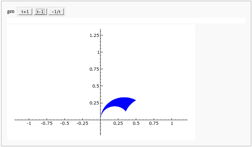
| def _(gen = selector(['t+1', 't-1', '-1/t'], nrows=1)): | def _(gen = selector(['t+1', 't-1', '-1/t'], buttons=True,nrows=1)): |
Contents
Integer Factorization
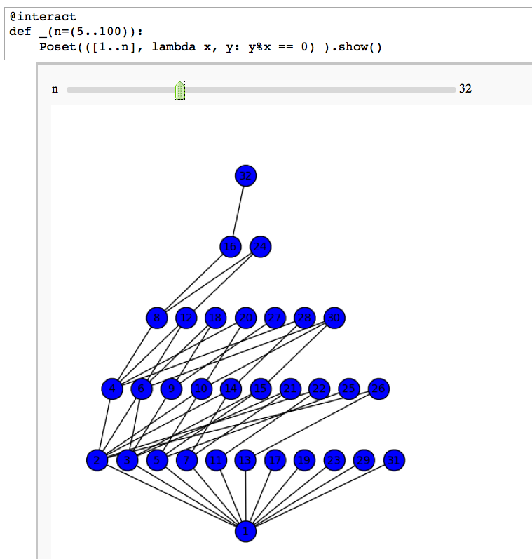
Divisibility Poset
by William Stein
Factor Trees
by William Stein
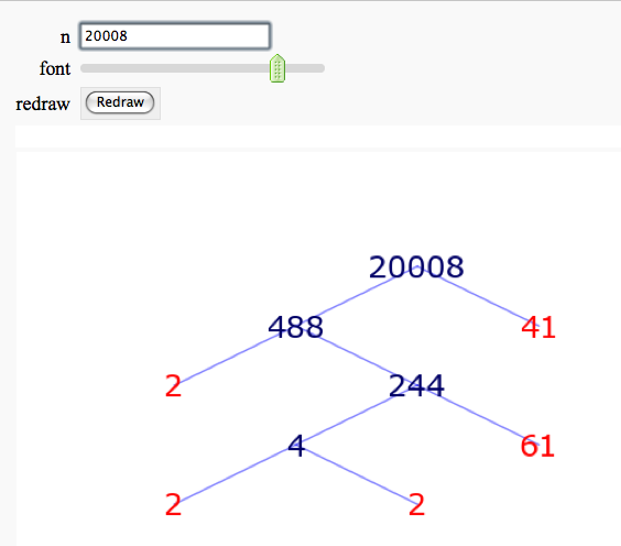
More complicated demonstration using Mathematica: http://demonstrations.wolfram.com/FactorTrees/
Factoring an Integer
by Timothy Clemans
Sage implementation of the Mathematica demonstration of the same name. http://demonstrations.wolfram.com/FactoringAnInteger/
Prime Numbers
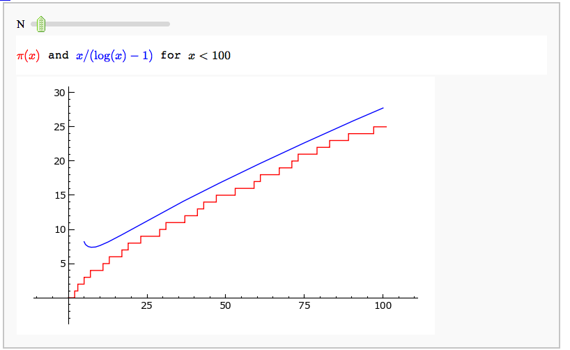
Illustrating the prime number theorem
by William Stein
Prime Spiral - Square FIXME
by David Runde
Prime Spiral - Polar
by David Runde
Modular Forms
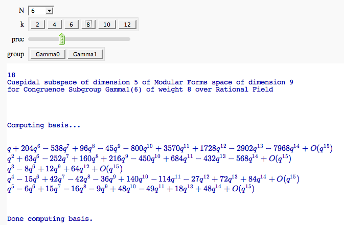
Computing modular forms
by William Stein
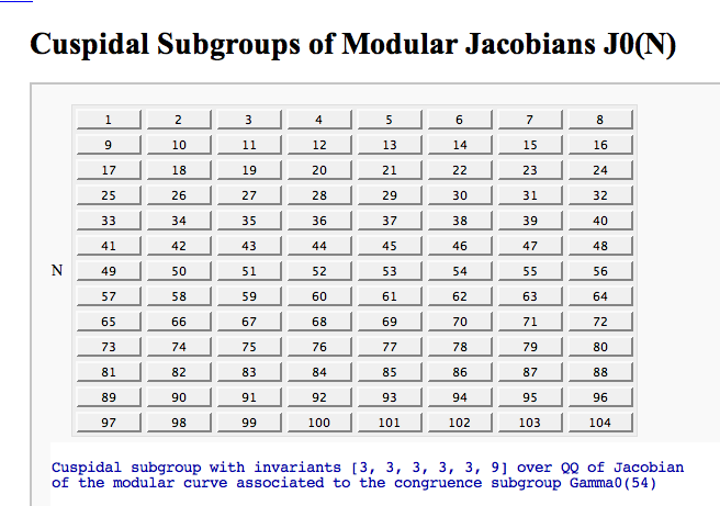
Computing the cuspidal subgroup
by William Stein
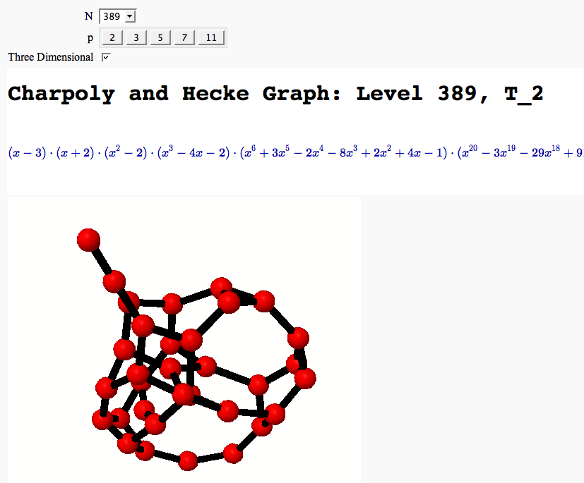
A Charpoly and Hecke Operator Graph
by William Stein
Modular Arithmetic
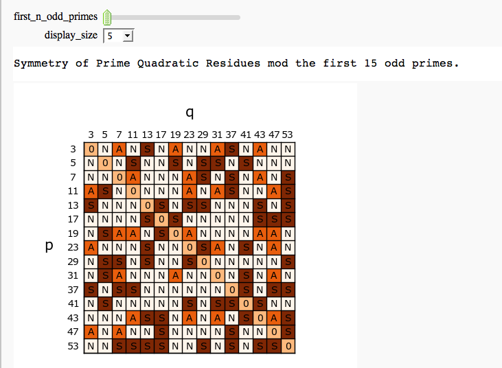
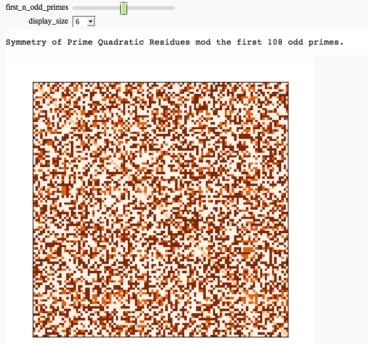
Quadratic Residue Table FIXME
by Emily Kirkman
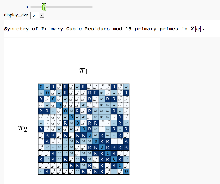
Cubic Residue Table FIXME
by Emily Kirkman
Cyclotomic Fields
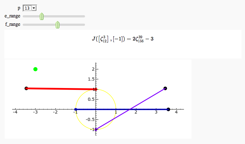
Gauss and Jacobi Sums in Complex Plane
by Emily Kirkman
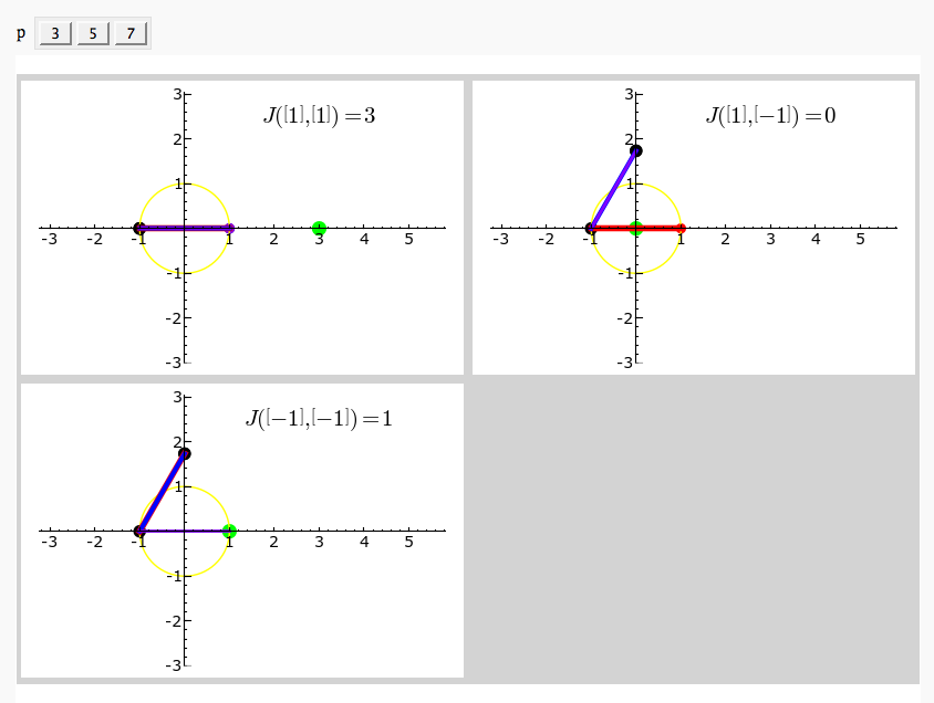
Exhaustive Jacobi Plotter
by Emily Kirkman
Elliptic Curves
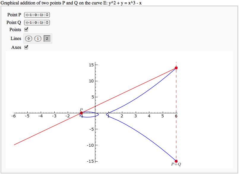
Adding points on an elliptic curve
by David Møller Hansen
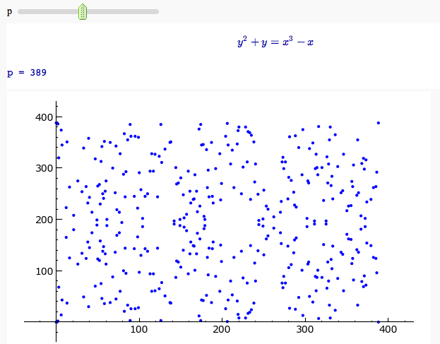
Plotting an elliptic curve over a finite field
Cryptography
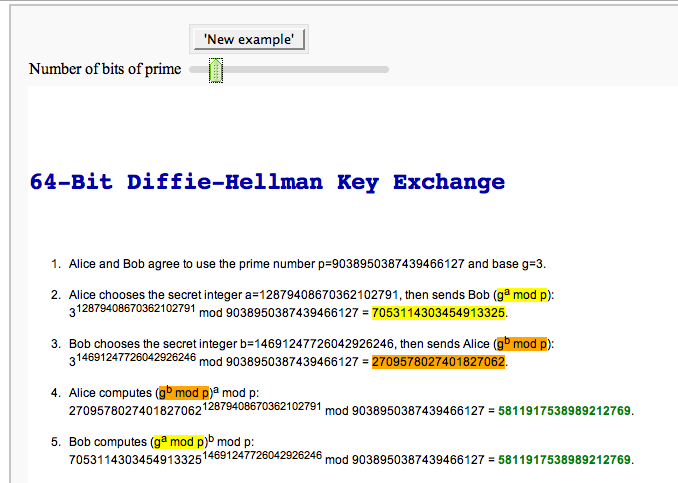
The Diffie-Hellman Key Exchange Protocol
by Timothy Clemans and William Stein
Other
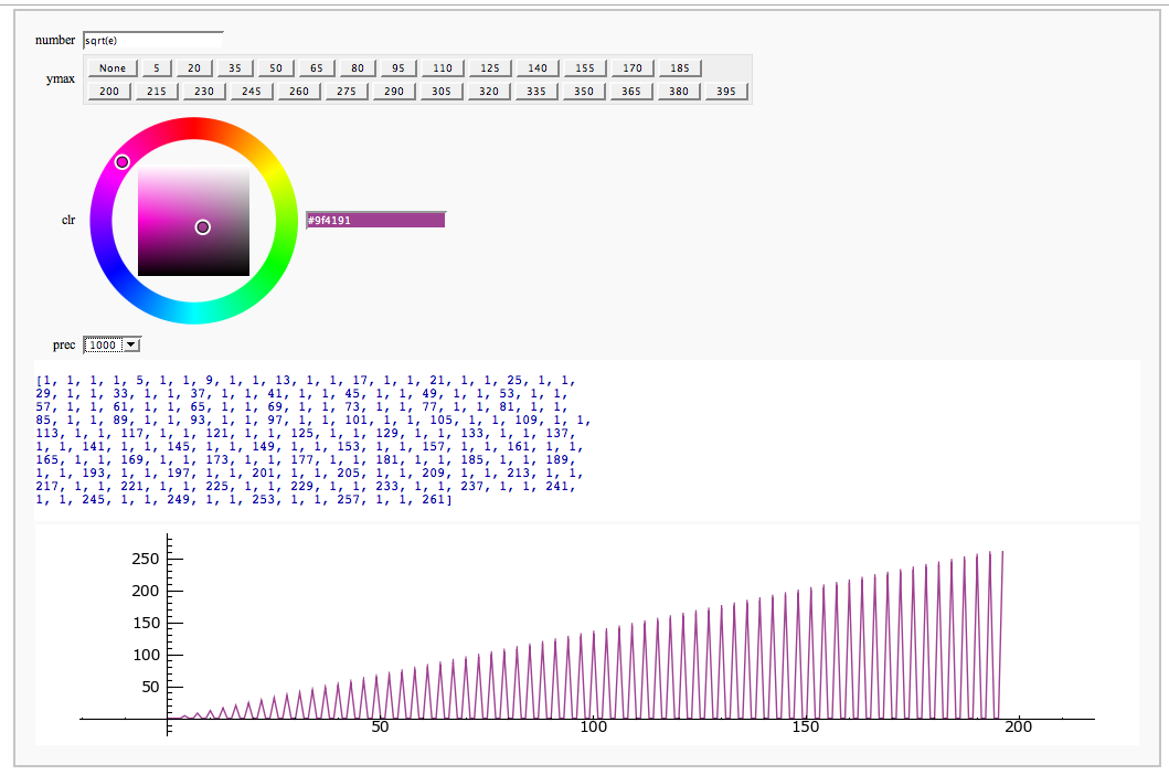
Continued Fraction Plotter
by William Stein
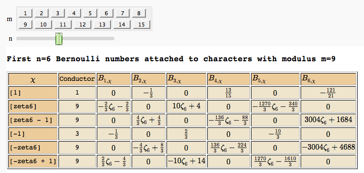
Computing Generalized Bernoulli Numbers
by William Stein (Sage-2.10.3)
Fundamental Domains of SL_2(ZZ)
by Robert Miller
