|
Size: 7542
Comment:
|
Size: 10742
Comment: py3 print
|
| Deletions are marked like this. | Additions are marked like this. |
| Line 2: | Line 2: |
| goto [:interact:interact main page] == Stock Market data, fetched from Yahoo and Google == |
goto [[interact|interact main page]] <<TableOfContents>> == Stock Market data, fetched from Yahoo and Google FIXME == |
| Line 7: | Line 9: |
| {{{ | (Need to fix plotting warnings as well as some stocks give index errors (like bsc, etc.) {{{#!sagecell |
| Line 124: | Line 128: |
| attachment:stocks.png | {{attachment:stocks.png}} |
| Line 130: | Line 134: |
| {{{ | {{{#!sagecell from scipy.optimize import leastsq |
| Line 133: | Line 138: |
| import time current_year = time.localtime().tm_year |
|
| Line 142: | Line 149: |
| trdf = RealField(16) @interact def mauna_loa_co2(start_date = slider(1958,2010,1,1958), end_date = slider(1958, 2010,1,2009)): |
npi = RDF(pi) @interact(layout=[['start_date'],['end_date'],['show_linear_fit','show_nonlinear_fit']]) def mauna_loa_co2(start_date = slider(1958,current_year,1,1958), end_date = slider(1958, current_year,1,current_year-1), show_linear_fit = checkbox(default=True), show_nonlinear_fit = checkbox(default=False)): |
| Line 147: | Line 154: |
| sel_data = [[q[2],q[4]] for q in datalines if start_date < q[2] < end_date] | html(htmls1+htmls2) sel_data = [[q[2],q[4]] for q in datalines if start_date <= q[2] <= end_date] outplot = list_plot(sel_data, plotjoined=True, rgbcolor=(1,0,0)) if show_nonlinear_fit: def powerlaw(t,a): return sel_data[0][1] + a[0]*(t-sel_data[0][0])^(a[1]) def res_fun(a): return [q[1]-powerlaw(q[0],a) for q in sel_data] def fitcos(t,a): return a[0]*cos(t*2*npi+a[1])+a[2]*cos(t*4*npi+a[3]) def res_fun2(a): return [q[1]-fitcos(q[0],a) for q in resids] a1 = leastsq(res_fun,[1/2.4,1.3])[0] resids = [[q[0],q[1] - powerlaw(q[0],a1)] for q in sel_data] a2 = leastsq(res_fun2, [3,0,1,0])[0] r2_plot = list_plot([[q[0],powerlaw(q[0],a1)+fitcos(q[0],a2)] for q in resids], rgbcolor='green',plotjoined=True) outplot = outplot + r2_plot var('t') formula1 = '%.2f+%.2f(t - %d)^%.2f'%(sel_data[0][1],a1[0],sel_data[0][0],a1[1]) formula2 = '%.2fcos(2 pi t + %.2f)+%.2f cos(4 pi t + %.2f)'%(a2[0],a2[1],a2[2],a2[3]) html('Nonlinear fit: <br>%s<br>'%(formula1+'+'+formula2)) if show_linear_fit: slope, intercept, r, ttprob, stderr = Stat.linregress(sel_data) outplot = outplot + plot(slope*x+intercept,start_date,end_date) html('Linear regression slope: %.2f ppm/year; correlation coefficient: %.2f'%(slope,r)) var('x,y') |
| Line 150: | Line 182: |
| slope, intercept, r, ttprob, stderr = Stat.linregress(sel_data) html(htmls1+htmls2+'<h4>Linear regression slope: ' + str(trdf(slope)) + ' ppm/year; correlation coefficient: ' + str(trdf(r)) + '</h4>') var('x,y') show(list_plot(sel_data, plotjoined=True, rgbcolor=(1,0,0)) + plot(slope*x+intercept,start_date,end_date), xmin = start_date, ymin = c_min-2, axes = True, xmax = end_date, ymax = c_max+3, frame = False) }}} attachment:co2c.png |
show(outplot, xmin = start_date, ymin = c_min-2, axes = True, xmax = end_date, ymax = c_max+3, frame = False) }}} {{attachment:co2c.png}} == Arctic sea ice extent data plot, fetched from NSIDC == by Marshall Hampton {{{#!sagecell import urllib2, csv months = ['Jan','Feb','Mar','Apr','May','Jun','Jul','Aug','Sep','Oct','Nov','Dec'] longmonths = ['January','February','March','April','May','June','July','August','September','October','November','December'] @interact def iceplotter(month = selector(zip(range(1,13),longmonths),default = (4, 'April'),label="Month")): month_str = months[month-1] + '/N_%02d_area.txt'%(month) dialect=csv.excel dialect.skipinitialspace = True icedata_f = urllib2.urlopen('ftp://sidads.colorado.edu/DATASETS/NOAA/G02135/%s'%month_str) cr = csv.reader(icedata_f,delimiter=' ', dialect=dialect) icedata = list(cr) icedata = [x for x in icedata[1:] if len(x)==6 and N(x[5])>0] lp = list_plot([[N(x[0]),N(x[4])] for x in icedata]) def lin_regress(xdata, ydata): xmean = N(mean(xdata)) ymean = N(mean(ydata)) xm = vector(RDF,[q-xmean for q in xdata]) ym = vector(RDF,[q-ymean for q in ydata]) xy = xm.inner_product(ym) xx = xm.inner_product(xm) slope = xy/xx intercept = ymean - slope*xmean return slope, intercept years = [N(x[0]) for x in icedata] ice = [N(x[4]) for x in icedata] slope, inter = lin_regress(years,ice) reg = plot(lambda x:slope*x+inter,(min(years),max(years))) html('<h3>Extent of Arctic sea ice coverage in %s, %d - %d</h3>'%(longmonths[month-1],min(years),max(years))) html('Data from the <a href="http://nsidc.org/">National Snow and Ice Data Center</a>') show(lp+reg, figsize = [7,4]) }}} {{attachment:seaice.png}} |
| Line 160: | Line 229: |
| {{{ | {{{#!sagecell |
| Line 171: | Line 240: |
| print url | print(url) |
| Line 174: | Line 243: |
| attachment:interact_with_google_chart_api.png | {{attachment:interact_with_google_chart_api.png}} |
Sage Interactions - Web applications
goto interact main page
Contents
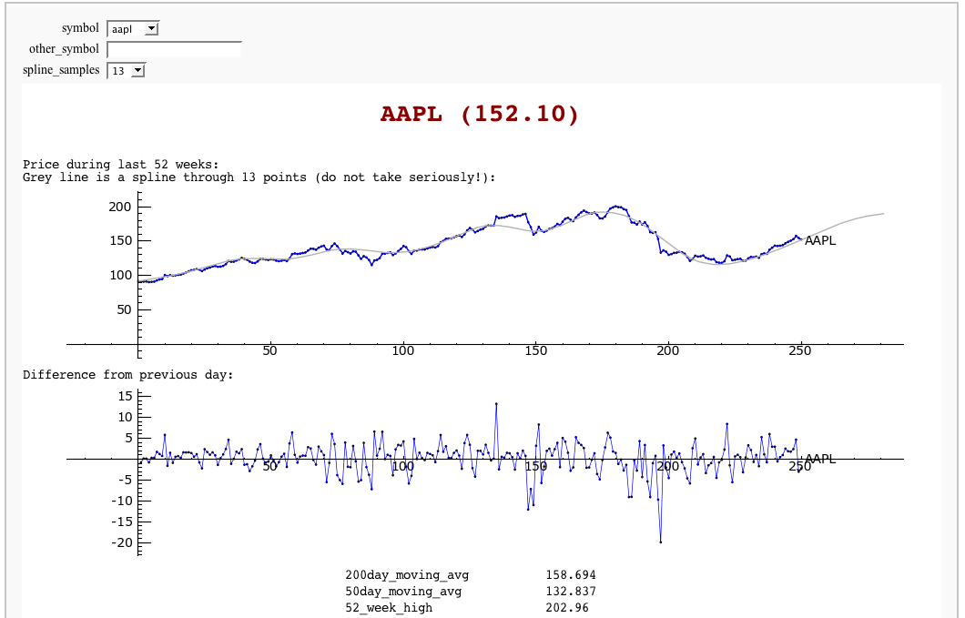
Stock Market data, fetched from Yahoo and Google FIXME
by William Stein
(Need to fix plotting warnings as well as some stocks give index errors (like bsc, etc.)

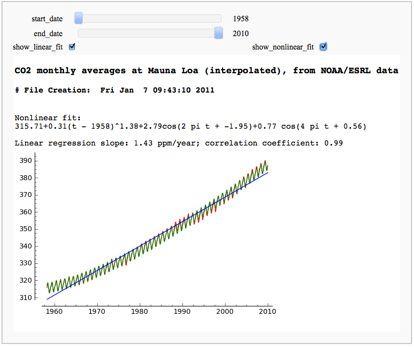
CO2 data plot, fetched from NOAA
by Marshall Hampton
While support for R is rapidly improving, scipy.stats has a lot of useful stuff too. This only scratches the surface.

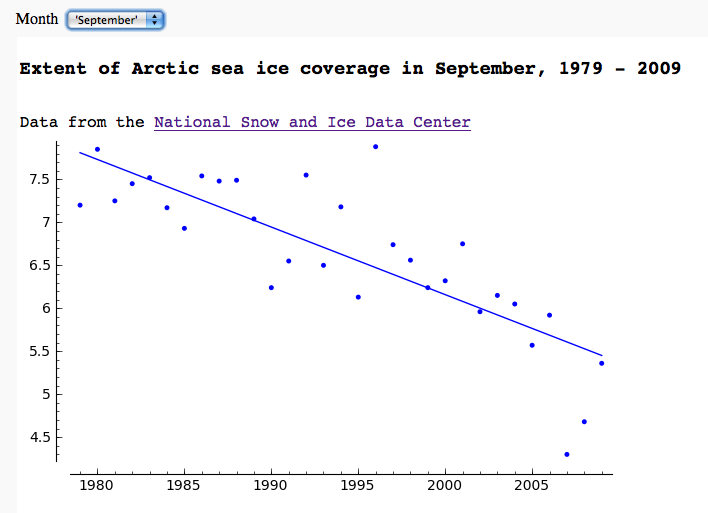
Arctic sea ice extent data plot, fetched from NSIDC
by Marshall Hampton

Pie Chart from the Google Chart API
by Harald Schilly

