Size: 10603
Comment:
|
Size: 10643
Comment:
|
Deletions are marked like this. | Additions are marked like this. |
Line 9: | Line 9: |
{{{ | {{{#!sagecell |
Line 132: | Line 132: |
{{{ | {{{#!sagecell |
Line 187: | Line 187: |
{{{ | {{{#!sagecell |
Line 227: | Line 227: |
{{{ | {{{#!sagecell |
Sage Interactions - Web applications
goto interact main page
Contents
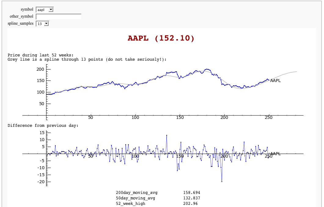
Stock Market data, fetched from Yahoo and Google
by William Stein
xxxxxxxxxx
import urllib
class Day:
def __init__(self, date, open, high, low, close, volume):
self.date = date
self.open=float(open); self.high=float(high); self.low=float(low); self.close=float(close)
self.volume=int(volume)
def __repr__(self):
return '%10s %4.2f %4.2f %4.2f %4.2f %10d'%(self.date, self.open, self.high,
self.low, self.close, self.volume)
class Stock:
def __init__(self, symbol):
self.symbol = symbol.upper()
def __repr__(self):
return "%s (%s)"%(self.symbol, self.yahoo()['price'])
def yahoo(self):
url = 'http://finance.yahoo.com/d/quotes.csv?s=%s&f=%s' % (self.symbol, 'l1c1va2xj1b4j4dyekjm3m4rr5p5p6s7')
values = urllib.urlopen(url).read().strip().strip('"').split(',')
data = {}
data['price'] = values[0]
data['change'] = values[1]
data['volume'] = values[2]
data['avg_daily_volume'] = values[3]
data['stock_exchange'] = values[4]
data['market_cap'] = values[5]
data['book_value'] = values[6]
data['ebitda'] = values[7]
data['dividend_per_share'] = values[8]
data['dividend_yield'] = values[9]
data['earnings_per_share'] = values[10]
data['52_week_high'] = values[11]
data['52_week_low'] = values[12]
data['50day_moving_avg'] = values[13]
data['200day_moving_avg'] = values[14]
data['price_earnings_ratio'] = values[15]
data['price_earnings_growth_ratio'] = values[16]
data['price_sales_ratio'] = values[17]
data['price_book_ratio'] = values[18]
data['short_ratio'] = values[19]
return data
def historical(self):
try:
return self.__historical
except AttributeError:
pass
symbol = self.symbol
def get_data(exchange):
name = get_remote_file('http://finance.google.com/finance/historical?q=%s:%s&output=csv'%(exchange, symbol.upper()),
verbose=False)
return open(name).read()
R = get_data('NASDAQ')
if "Bad Request" in R:
R = get_data("NYSE")
R = R.splitlines()
headings = R[0].split(',')
self.__historical = []
try:
for x in reversed(R[1:]):
date, opn, high, low, close, volume = x.split(',')
self.__historical.append(Day(date, opn,high,low,close,volume))
except ValueError:
pass
self.__historical = Sequence(self.__historical,cr=True,universe=lambda x:x)
return self.__historical
def plot_average(self, spline_samples=10):
d = self.historical()
if len(d) == 0:
return text('no historical data at Google Finance about %s'%self.symbol, (0,3))
avg = list(enumerate([(z.high+z.low)/2 for z in d]))
P = line(avg) + points(avg, rgbcolor='black', pointsize=4) + \
text(self.symbol, (len(d)*1.05, d[-1].low), horizontal_alignment='right', rgbcolor='black')
if spline_samples > 0:
k = 250//spline_samples
spl = spline([avg[i*k] for i in range(len(d)//k)] + [avg[-1]])
P += plot(spl, (0,len(d)+30), color=(0.7,0.7,0.7))
P.xmax(260)
return P
def plot_diff(self):
d = self.historical()
if len(d) == 0:
return text('no historical data at Google Finance about %s'%self.symbol, (0,3))
diff = []
for i in range(1, len(d)):
z1 = d[i]; z0 = d[i-1]
diff.append((i, (z1.high+z1.low)/2 - (z0.high + z0.low)/2))
P = line(diff,thickness=0.5) + points(diff, rgbcolor='black', pointsize=4) + \
text(self.symbol, (len(d)*1.05, 0), horizontal_alignment='right', rgbcolor='black')
P.xmax(260)
return P
symbols = ['bsc', 'vmw', 'sbux', 'aapl', 'amzn', 'goog', 'wfmi', 'msft', 'yhoo', 'ebay', 'java', 'rht', ]; symbols.sort()
stocks = dict([(s,Stock(s)) for s in symbols])
def data(symbol = symbols, other_symbol='', spline_samples=(8,[0..15])):
if other_symbol != '':
symbol = other_symbol
S = Stock(symbol)
html('<h1 align=center><font color="darkred">%s</font></h1>'%S)
S.plot_average(spline_samples).save('avg.png', figsize=[10,2])
S.plot_diff().save('diff.png', figsize=[10,2])
Y = S.yahoo()
k = Y.keys(); k.sort()
html('Price during last 52 weeks:<br>Grey line is a spline through %s points (do not take seriously!):<br> <img src="cell://avg.png">'%spline_samples)
html('Difference from previous day:<br> <img src="cell://diff.png">')
html('<table align=center>' + '\n'.join('<tr><td>%s</td><td>%s</td></tr>'%(k[i], Y[k[i]]) for i in range(len(k))) + '</table>')
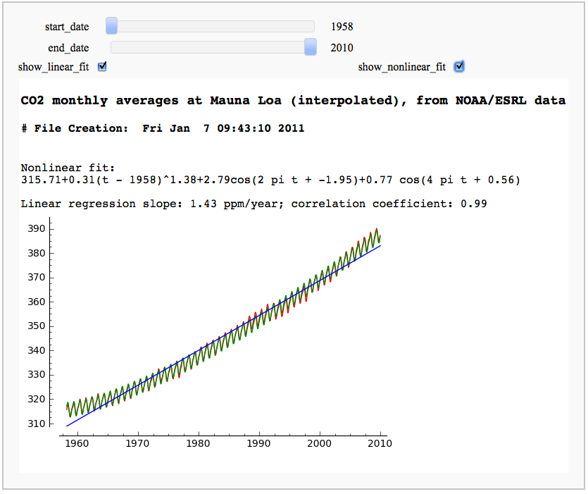
CO2 data plot, fetched from NOAA
by Marshall Hampton
While support for R is rapidly improving, scipy.stats has a lot of useful stuff too. This only scratches the surface.
xxxxxxxxxx
from scipy.optimize import leastsq
import urllib2 as U
import scipy.stats as Stat
import time
current_year = time.localtime().tm_year
co2data = U.urlopen('ftp://ftp.cmdl.noaa.gov/ccg/co2/trends/co2_mm_mlo.txt').readlines()
datalines = []
for a_line in co2data:
if a_line.find('Creation:') != -1:
cdate = a_line
if a_line[0] != '#':
temp = a_line.replace('\n','').split(' ')
temp = [float(q) for q in temp if q != '']
datalines.append(temp)
npi = RDF(pi)
layout=[['start_date'],['end_date'],['show_linear_fit','show_nonlinear_fit']]) (
def mauna_loa_co2(start_date = slider(1958,current_year,1,1958), end_date = slider(1958, current_year,1,current_year-1), show_linear_fit = checkbox(default=True), show_nonlinear_fit = checkbox(default=False)):
htmls1 = '<h3>CO2 monthly averages at Mauna Loa (interpolated), from NOAA/ESRL data</h3>'
htmls2 = '<h4>'+cdate+'</h4>'
html(htmls1+htmls2)
sel_data = [[q[2],q[4]] for q in datalines if start_date <= q[2] <= end_date]
outplot = list_plot(sel_data, plotjoined=True, rgbcolor=(1,0,0))
if show_nonlinear_fit:
def powerlaw(t,a):
return sel_data[0][1] + a[0]*(t-sel_data[0][0])^(a[1])
def res_fun(a):
return [q[1]-powerlaw(q[0],a) for q in sel_data]
def fitcos(t,a):
return a[0]*cos(t*2*npi+a[1])+a[2]*cos(t*4*npi+a[3])
def res_fun2(a):
return [q[1]-fitcos(q[0],a) for q in resids]
a1 = leastsq(res_fun,[1/2.4,1.3])[0]
resids = [[q[0],q[1] - powerlaw(q[0],a1)] for q in sel_data]
a2 = leastsq(res_fun2, [3,0,1,0])[0]
r2_plot = list_plot([[q[0],powerlaw(q[0],a1)+fitcos(q[0],a2)] for q in resids], rgbcolor='green',plotjoined=True)
outplot = outplot + r2_plot
var('t')
formula1 = '%.2f+%.2f(t - %d)^%.2f'%(sel_data[0][1],a1[0],sel_data[0][0],a1[1])
formula2 = '%.2fcos(2 pi t + %.2f)+%.2f cos(4 pi t + %.2f)'%(a2[0],a2[1],a2[2],a2[3])
html('Nonlinear fit: <br>%s<br>'%(formula1+'+'+formula2))
if show_linear_fit:
slope, intercept, r, ttprob, stderr = Stat.linregress(sel_data)
outplot = outplot + plot(slope*x+intercept,start_date,end_date)
html('Linear regression slope: %.2f ppm/year; correlation coefficient: %.2f'%(slope,r))
var('x,y')
c_max = max([q[1] for q in sel_data])
c_min = min([q[1] for q in sel_data])
show(outplot, xmin = start_date, ymin = c_min-2, axes = True, xmax = end_date, ymax = c_max+3, frame = False)
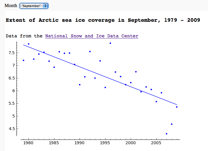
Arctic sea ice extent data plot, fetched from NSIDC
by Marshall Hampton
xxxxxxxxxx
import urllib2, csv
months = ['Jan','Feb','Mar','Apr','May','Jun','Jul','Aug','Sep','Oct','Nov','Dec']
longmonths = ['January','February','March','April','May','June','July','August','September','October','November','December']
def iceplotter(month = selector(zip(range(1,13),longmonths),default = (4, 'April'),label="Month")):
month_str = months[month-1] + '/N_%02d_area.txt'%(month)
dialect=csv.excel
dialect.skipinitialspace = True
icedata_f = urllib2.urlopen('ftp://sidads.colorado.edu/DATASETS/NOAA/G02135/%s'%month_str)
cr = csv.reader(icedata_f,delimiter=' ', dialect=dialect)
icedata = list(cr)
icedata = [x for x in icedata[1:] if len(x)==6 and N(x[5])>0]
lp = list_plot([[N(x[0]),N(x[4])] for x in icedata])
def lin_regress(xdata, ydata):
xmean = N(mean(xdata))
ymean = N(mean(ydata))
xm = vector(RDF,[q-xmean for q in xdata])
ym = vector(RDF,[q-ymean for q in ydata])
xy = xm.inner_product(ym)
xx = xm.inner_product(xm)
slope = xy/xx
intercept = ymean - slope*xmean
return slope, intercept
years = [N(x[0]) for x in icedata]
ice = [N(x[4]) for x in icedata]
slope, inter = lin_regress(years,ice)
reg = plot(lambda x:slope*x+inter,(min(years),max(years)))
html('<h3>Extent of Arctic sea ice coverage in %s, %d - %d</h3>'%(longmonths[month-1],min(years),max(years)))
html('Data from the <a href="http://nsidc.org/">National Snow and Ice Data Center</a>')
show(lp+reg, figsize = [7,4])
Pie Chart from the Google Chart API
by Harald Schilly
xxxxxxxxxx
# Google Chart API: http://code.google.com/apis/chart
import urllib2 as inet
from pylab import imshow
def gChart(title="Google Chart API plots Pie Charts!", color1=Color('purple'), color2=Color('black'), color3=Color('yellow'), val1=slider(0,1,.05,.5), val2=slider(0,1,.05,.3), val3=slider(0,1,.05,0.1), label=("Maths Physics Chemistry")):
url = "http://chart.apis.google.com/chart?cht=p3&chs=600x300"
url += '&chtt=%s&chts=000000,25'%title.replace(" ","+")
url += '&chco=%s'%(','.join([color1.html_color()[1:],color2.html_color()[1:],color3.html_color()[1:]]))
url += '&chl=%s'%label.replace(" ","|")
url += '&chd=t:%s'%(','.join(map(str,[val1,val2,val3])))
print url
html('<div style="border:3px dashed;text-align:center;padding:50px 0 50px 0"><img src="%s"></div>'%url)